Diagnostics: maturity, convergence, regime

Overview

Before reading a projected loss ratio off a fit, it pays to ask three questions about the triangle that feeds it. lossratio answers them with three diagnostics, each on its own axis:

Tool	Question	Result	Axis
`detect_maturity()` ( $k^*$ )	When are link factors reproducible?	a dev value	development period
`detect_convergence()` ( $k^{**}$ )	When does the LR estimate stop revising?	a dev value	development period
`detect_regime()`	Are underwriting cohorts homogeneous?	cohort groups	underwriting period

In P&C run-off these three properties tend to coincide; in long-duration health insurance they must be verified independently. This vignette walks them in dependency order — maturity, then convergence (which builds on maturity), then regime — and closes with how a detected regime is fed back into fit_* as a data filter.

All examples use the bundled experience dataset’s surgery coverage, which carries a synthetic 2024-04 regime change so the detectors have a clear signal to find.

library(lossratio)
data(experience)
tri_sur <- as_triangle(
  experience[coverage == "surgery"],
  groups   = "coverage",
  cohort   = "uy_m",
  calendar = "cy_m",
  loss     = "incr_loss",
  premium  = "incr_premium"
)

Maturity detection

The maturity point is the development link beyond which age-to-age factors are stable enough to trust for chain-ladder projection. It is used internally by fit_ratio(method = "sa") to switch from the exposure-driven (ED) region to the chain-ladder (CL) region.

detect_maturity() takes a Triangle directly — the underlying single-variable Link and its WLS summary are built internally:

mat <- detect_maturity(
  tri_sur,
  loss            = "loss",
  max_cv          = 0.15,    # CV must be below this
  max_rse         = 0.05,    # RSE must be below this
  min_valid_ratio = 0.5,     # at least 50% finite cohorts at the link
  min_n_valid     = 3L,      # at least 3 finite cohorts
  min_run         = 1L       # at least 1 consecutive mature link
)

print(mat)
#> Key: <coverage>
#>    coverage ata_from change ata_link     mean   median       wt        cv
#>      <char>    <num>  <num>   <char>    <num>    <num>    <num>     <num>
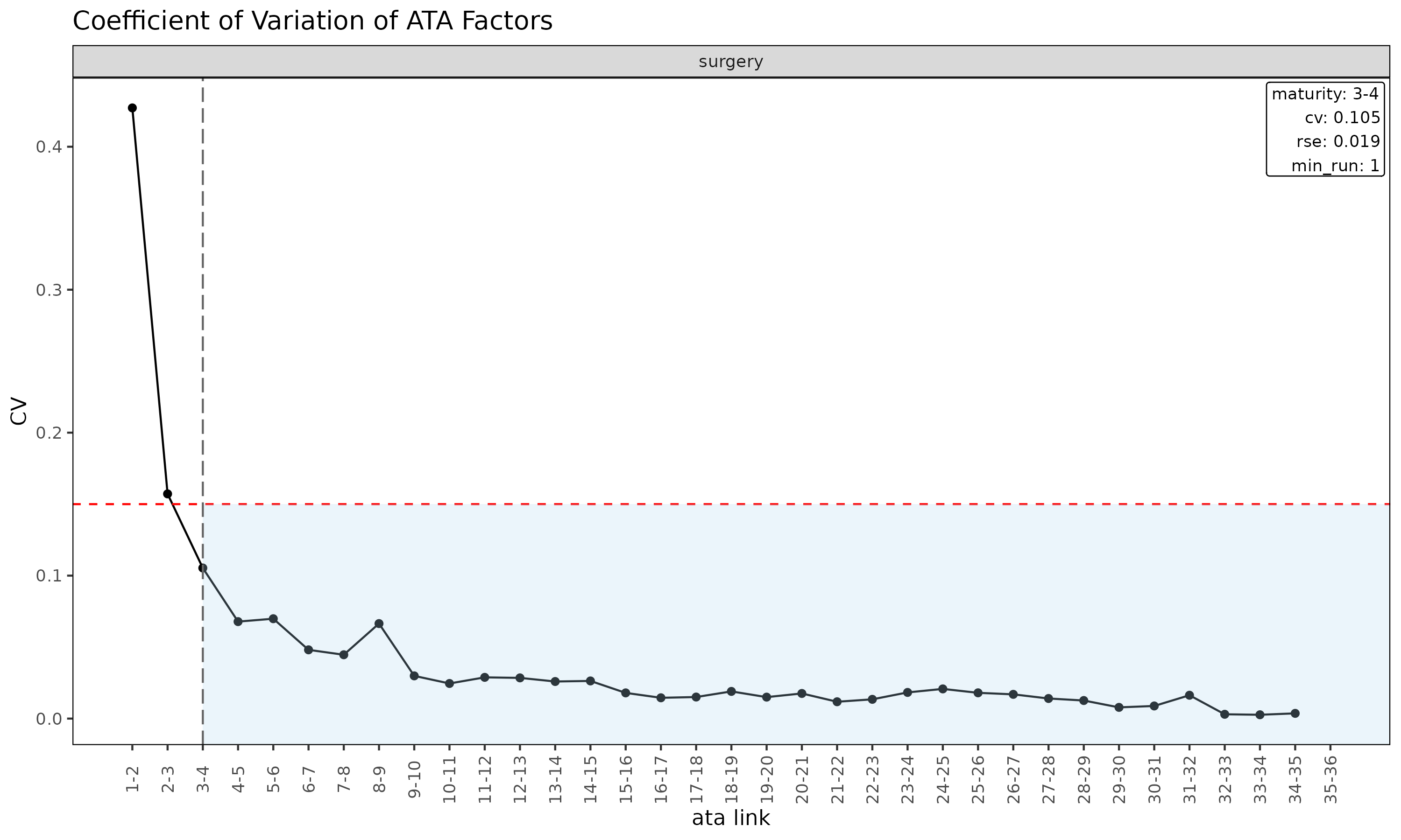
#> 1:  surgery        3      4      3-4 1.434507 1.400098 1.417706 0.1053282
#>           f       f_se        rse    sigma n_cohorts n_valid n_inf n_nan
#>       <num>      <num>      <num>    <num>     <num>   <num> <num> <num>
#> 1: 1.417706 0.02651852 0.01870522 1372.883        33      33     0     0
#>    valid_ratio
#>          <num>
#> 1:           1

The result is a row per group with the first development link satisfying all thresholds, carrying that link’s full statistics. The threshold arguments are also stored as attributes on the returned Maturity object.

Threshold semantics

max_cv — coefficient of variation of the observed ATA factors at the link. Caps relative spread regardless of alpha.
max_rse — relative standard error of the WLS-estimated factor f. Captures parameter uncertainty rather than residual spread.
min_valid_ratio — minimum share of cohorts with a finite ATA at the link. Guards against links where most observations are zero / NA / Inf.
min_n_valid — minimum count of finite cohorts at the link. An absolute floor for thin-data tails.
min_run — minimum number of consecutive mature links. With min_run = 1L (default) the first qualifying link wins; setting it to 2L or higher requires sustained stability.

Tune these to the portfolio’s volatility profile. Tight thresholds (e.g. max_cv = 0.05) push maturity later; loose thresholds push it earlier. The link diagnostic plot makes the result easy to read — each CV gets its own panel and a vertical line marks the maturity point where CV first drops below max_cv:

plot(as_link(tri_sur, loss = "loss"), type = "cv")

Use in fitting

detect_maturity() is also called internally by fit_ata(), fit_cl(), and fit_ratio(method = "sa") via the maturity argument. It accepts four forms:

NULL — no detection (worker default for standalone calls).
a pre-built Maturity object — from detect_maturity(), or from maturity_at() for a manual override.
"auto" — internal detect_maturity() with defaults (the default for fit_ratio(method = "sa") and fit_loss()).
a function of one triangle returning a Maturity — typically maturity_spec(), which forwards custom detection thresholds.

fit_ata(tri_sur, loss = "loss",
        maturity = maturity_spec(max_cv = 0.08, min_run = 2L))

fit_ratio(tri_sur, method = "sa",
          maturity = maturity_spec(max_cv = 0.08))

For fit_ratio(method = "sa") the detected maturity point determines the dev at which the projection switches from ED (early dev) to CL (later dev).

Convergence detection

Maturity answers “from which development period are link factors $f_k$ reproducible across cohorts?”. That is necessary for chain-ladder projection but not sufficient for declaring a portfolio’s projected loss ratio converged. In long-duration health insurance both $f_k \to 1$ and $g_k \to 0$ arise mechanically as cumulative denominators grow — independent of whether the underlying experience has actually settled. A criterion built on those quantities passes automatically with $k$ , not because of true convergence (the inertia failure mode).

detect_convergence() detects the convergence point $k^{**}$ — the first dev $k \ge k^*$ at which the projected portfolio loss ratio is observed to be stable, in a sense the user picks via method =. It is the natural counterpart to $k^*$ :

$k^*$ (detect_maturity()) marks where link factors $f_k$ become reproducible.
$k^{**}$ marks where the projection itself stops moving with new data.

Long-duration health portfolios may cross $k^*$ early yet remain far from $k^{**}$ .

The four stability methods

Convergence cannot be measured asymptotically from finite data, only observed up to the maximum available dev dev_max ( $K_{\max}$ ). The detector runs a rolling backtest() over a sequence of candidate dev points dev_cand $\in [k^*, K_{\max}-2]$ , builds the projected ultimate LR path ratio at each one, then evaluates four stability metrics on that path. The method = argument selects which metric defines conv_k; all four are returned for inspection regardless of the choice.

Method	Metric	Captures	Misses
`"window"`	range of `ratio` over the next `window` valuations	local stability (no zig-zag)	slow monotone drift below `max_drift` per window
`"tail"` (default)	range of `ratio` over `[k, K_{\max}]`	global stability up to `dev_max`; catches monotone drift	needs $\ge 2$ tail points; first-pass is conservative (later than `"window"`)
`"slope"`	$\\|\hat\beta_k\\|$ , OLS slope of `ratio ~ k` on `[k, K_{\max}]`	systematic trend (signed direction)	oscillation that averages out to zero slope
`"all"`	intersection of `"window"` + `"tail"` + `"slope"`	every shape above	(strictest)

Across all methods a cross-cohort dispersion clause dispersion[i] < max_dispersion is required in addition — incremental loss ratios at that dev must agree across cohorts (computed via the robust $\hat{D}_v$ metric). The constant $1.4826 \approx 1 / \Phi^{-1}(0.75)$ inside dispersion is the standard MAD $\to\sigma$ correction, so $\hat{D}_k$ reads as a robust, outlier-resistant coefficient of variation of incremental LR.

Why not an SE-normalised criterion? Earlier versions of this detector implemented $R_k < c \cdot \hat{SE}^{\mathrm{param}}_k$ from the original methodology paper (Section 11; the paper uses $v$ instead of $k$ , same axis). On large portfolios that form is structurally broken: $\hat{SE}^{\mathrm{param}}$ shrinks as $1/\sqrt{n}$ while $R_k$ has a numerical noise floor (~ $10^{-3}$ LR units), so the ratio diverges and the criterion never fires — even on synthetic data that is visibly stable. The drift-based methods replace SE-normalisation with a data-size-independent threshold.

Notation

Standard chain-ladder convention: $i$ indexes cohort (origin period), $k$ indexes development period. detect_maturity() returns $k^*$ , detect_convergence() returns $k^{**}$ — both live on the same $k$ axis.

Code	Math	Meaning
`dev_max`	$K_{\max}$	Maximum observable dev (a scalar)
`dev_cand`	$k \in [k^*, K_{\max}-2]$	Integer vector of candidate dev points
`ratio[i]`	$LR_k$	Portfolio LR projection at dev = `dev_cand[i]`
`revision[i]`	$R_k = \\|LR_k - LR_{k-1}\\|$	Adjacent-step revision (diagnostic only)
`drift_window[i]`	$\max - \min$ over $[k, k+W-1]$	Local window range
`drift_tail[i]`	$\max - \min$ over $[k, K_{\max}]$	Tail range (global stability)
`slope[i]`	$\hat\beta_k$	OLS slope on $[k, K_{\max}]$
`dispersion[i]`	$\hat{D}_k$	Robust cross-cohort spread of incremental LR
`mat_k`	$k^*$	Maturity point (lower bound on candidates)
`conv_k`	$k^{**}$	The detected convergence point

Basic usage

res <- detect_convergence(tri_sur)
print(res)

Mock output (no convergence detected on this run-off):

#> <Convergence>
#>   method     : tail
#>   conv_k     : NA
#>   mat_k      : 4
#>   dev_max    : 30
#>   candidates : 25
#>   passes :
#>     window :  0/25 (drift_window < 0.01  & dispersion < 0.15)
#>     tail   :  0/25 (drift_tail   < 0.01  & dispersion < 0.15)  <- method
#>     slope  :  0/25 (|slope|      < 0.001 & dispersion < 0.15)
#>     all    :  0/25 (window AND tail AND slope)

The summary data.table has one row per candidate dev with every metric and per-method pass flag:

head(summary(res), 6)

#>      dev ratio   revision  drift_window  drift_tail   slope  dispersion
#>    <int> <num>      <num>         <num>       <num>   <num>       <num>
#> 1:     4 0.62          NA          0.07        0.07   0.001        0.47
#> 2:     5 0.63        0.01          0.06        0.06   0.001        0.47
#> ...
#>    pass_window  pass_tail  pass_slope  pass
#>          <lgl>      <lgl>       <lgl> <lgl>
#> 1:       FALSE      FALSE       FALSE FALSE
#> 2:       FALSE      FALSE       FALSE FALSE

The Convergence object also reports the threshold parameters (max_drift, max_slope, max_dispersion, window, holdout_max, min_n_cohorts) and metadata attributes (groups, target, dispatcher).

How it works: rolling holdout refits

For each dev_cand[i], the function backtests the LR projection with holdout = dev_max - dev_cand[i] and extracts the portfolio LR. Calls are cached per holdout depth so we don’t redo work between adjacent candidates.

Example: with dev_max = 30, mat_k = 4, holdout_max = 13 — candidates are $k \in \{4, 5, \dots, 28\}$ (25 in total), but only $k$ with holdout = dev_max - k <= holdout_max get a finite ratio[i]. The rest are masked to NA. holdout_max defaults to max(window, floor((dev_max - mat_k) / 2)). Raising it widens the diagnostic window — at the cost of less data behind each refit and hence noisier ratio near the lower edge.

Plot

plot(res)

Five stacked panels share the dev axis:

ratio — the LR trajectory the metrics are computed from.
drift_window — the local-window metric, with horizontal guide at max_drift.
drift_tail — the tail metric, same guide.
|slope| — guide at max_slope.
dispersion — guide at max_dispersion.

Vertical guides mark mat_k (dashed) and conv_k (solid, only when non-NA). For each metric panel, points below the red dashed line pass that clause. The subtitle records the active method. This is also a quick way to see which clause is binding: any panel that hovers above its threshold blocks convergence under that method.

Threshold tuning

Argument	Default	Meaning
`method`	`"tail"`	Which stability metric defines `conv_k`.
`max_drift`	`0.01`	Drift cap on `drift_window` / `drift_tail`, in LR units. Raise (e.g. `0.02`–`0.05`) for noisier or longer-tail books.
`max_slope`	`1e-3`	$\\|\hat\beta_k\\|$ cap (LR per dev).
`max_dispersion`	`0.15`	Cross-cohort dispersion cap.
`window`	`5L`	Drift window length $W$ — number of consecutive valuations the `"window"` method scans. Does not affect `"tail"` or `"slope"`.
`min_n_cohorts`	`5L`	Below this cohort count, `dispersion` is `NA`.

Sweep max_drift to inspect sensitivity:

sapply(
  c(0.005, 0.01, 0.02, 0.05),
  function(d) detect_convergence(tri_sur, method = "tail", max_drift = d)$conv_k
)

max_dispersion below $\approx 0.05$ is difficult to attain in real portfolios because of single-period claim noise; values above $0.20$ usually indicate genuine cohort heterogeneity that warrants detect_regime() before further modelling.

Reserving caveat

The detected conv_k is stability observed up to dev_max, not an asymptotic guarantee. Future development past dev_max is unknown. Treat conv_k as a diagnostic for “from here on, what we observe is stable”, not as proof that the projection will not drift later.

For reserving applications:

Prefer method = "tail" (default) or "all" over "window". "window" will declare convergence prematurely on slow monotone drifts that fit under max_drift per window — exactly the silent-revision pattern that hurts reserves.
Always weigh the evidence span dev_max - conv_k. A conv_k near dev_max (say, span $< 5$ ) was confirmed by very few tail points; the same data might unconverge with one more diagonal.
Read the projected ultimate LR and its standard error from fit_ratio()$summary directly. detect_convergence() is a diagnostic, not an estimator; the reserve point estimate and uncertainty come from the fit object.

Limitations

detect_convergence() is a thin layer over repeated backtest() calls and inherits their constraints:

Identifiability: conv_k can be declared only when dev_max - mat_k >= window (or 2 for tail / slope). Short observation windows return NA for every method.
Model conditioning: the projected LR is computed by fit_ratio(), which internally composes fit_loss() (default method = "ed") and fit_premium(). Choices made inside that composition (loss method, regime filter, maturity argument) feed through to conv_k; pass loss_method =, loss_regime =, etc. through ... to override.
Portfolio aggregation: the portfolio LR aggregates per-group ultimates via premium weighting (sum(loss_ult) / sum(premium_ult)). Calendar-year shocks (regulatory changes, cost trend) can move every group together; the drift metrics will not separate that from genuine convergence.
Multi-group triangles: dispersion is currently collapsed across groups by median. When groups behave differently, running each group separately is recommended.

Regime detection

The two diagnostics above live on the development axis and assume the cohorts are homogeneous. When a portfolio undergoes a rate revision, coverage restructure, or underwriting overhaul, that assumption breaks: recent underwriting cohorts behave differently from earlier ones. Two questions follow:

Are recent underwriting cohorts behaving differently from earlier cohorts?
If so, when did the change happen?

In long-term insurance, cohort patterns most commonly break under one of four triggers:

Drastic premium adjustment — large up- or down-revision of rates.
Product coverage content change — restructuring of benefits, exclusions, or term.
Sum insured limit change — adjustment of per-policy maximum.
Underwriting guideline change — eligibility, declarations, or loading rule revisions.

A visual inspection of plot(tri_sur) can suggest that recent cohorts have lower early loss ratios than older ones, but eye-balling a bundle of trajectories is an unreliable way to locate a structural shift — especially when observation windows differ across cohorts.

detect_regime() answers both questions in one call — grouping underwriting cohorts into regimes (groups of cohorts that share similar loss dynamics) and reporting the break dates between groups. It treats each underwriting cohort as a feature vector (its trajectory over the first window development periods), orders cohorts by underwriting date, and applies a change-point or clustering method to the resulting multivariate sequence.

r <- detect_regime(tri_sur, method = "e_divisive")
r
#> <Regime>
#>   method    : e_divisive
#>   loss      : ratio
#>   treatment : segment_bridged
#>   window (window) : dev_m 1-4
#>   cohorts    : 33 analysed (3 dropped)
#>   regimes    : 2
#>   changes    : 24.07
#>   PC1 / PC2  : 75.6% / 18.9%

The window argument controls how many development periods define the cohort feature vector. Only cohorts observed for at least window periods are analysed; cohorts with shorter windows are dropped. Increasing window captures more of the trajectory but drops more recent cohorts. With the default window = "auto", a maturity-aware sweep picks the largest window that retains enough cohorts.

Summary and per-regime membership

summary(r)
#> Cohort regime detection summary
#>   method    : e_divisive
#>   loss      : ratio
#>   treatment : segment_bridged
#>   window    : dev_m 1-4
#>   cohorts   : 33 analysed (3 dropped)
#> 
#> Regimes (2):
#>   1: 23.01-24.06 (18 cohorts)
#>   2: 24.07-25.09 (15 cohorts)
#> 
#> Changes: 24.07

r$labels
#>     coverage     cohort      regime regime_id
#>       <char>     <Date>      <fctr>     <int>
#>  1:  surgery 2023-01-01 23.01-24.06         1
#>  2:  surgery 2023-02-01 23.01-24.06         1
#>  3:  surgery 2023-03-01 23.01-24.06         1
#>  4:  surgery 2023-04-01 23.01-24.06         1
#>  5:  surgery 2023-05-01 23.01-24.06         1
#>  6:  surgery 2023-06-01 23.01-24.06         1
#>  7:  surgery 2023-07-01 23.01-24.06         1
#>  8:  surgery 2023-08-01 23.01-24.06         1
#>  9:  surgery 2023-09-01 23.01-24.06         1
#> 10:  surgery 2023-10-01 23.01-24.06         1
#> 11:  surgery 2023-11-01 23.01-24.06         1
#> 12:  surgery 2023-12-01 23.01-24.06         1
#> 13:  surgery 2024-01-01 23.01-24.06         1
#> 14:  surgery 2024-02-01 23.01-24.06         1
#> 15:  surgery 2024-03-01 23.01-24.06         1
#> 16:  surgery 2024-04-01 23.01-24.06         1
#> 17:  surgery 2024-05-01 23.01-24.06         1
#> 18:  surgery 2024-06-01 23.01-24.06         1
#> 19:  surgery 2024-07-01 24.07-25.09         2
#> 20:  surgery 2024-08-01 24.07-25.09         2
#> 21:  surgery 2024-09-01 24.07-25.09         2
#> 22:  surgery 2024-10-01 24.07-25.09         2
#> 23:  surgery 2024-11-01 24.07-25.09         2
#> 24:  surgery 2024-12-01 24.07-25.09         2
#> 25:  surgery 2025-01-01 24.07-25.09         2
#> 26:  surgery 2025-02-01 24.07-25.09         2
#> 27:  surgery 2025-03-01 24.07-25.09         2
#> 28:  surgery 2025-04-01 24.07-25.09         2
#> 29:  surgery 2025-05-01 24.07-25.09         2
#> 30:  surgery 2025-06-01 24.07-25.09         2
#> 31:  surgery 2025-07-01 24.07-25.09         2
#> 32:  surgery 2025-08-01 24.07-25.09         2
#> 33:  surgery 2025-09-01 24.07-25.09         2
#>     coverage     cohort      regime regime_id
#>       <char>     <Date>      <fctr>     <int>

Visualisation

plot(r) produces a PCA scatter of cohort trajectories coloured by detected regime. If the regimes are well-separated in PCA space, the structural shift is visually confirmed:

plot(r)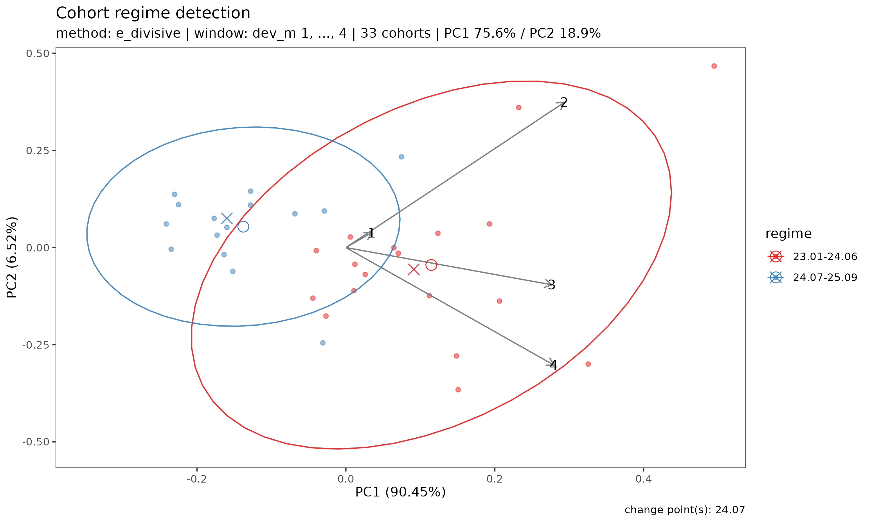

Arrows indicate the loadings of each development-period feature on the PC axes — useful for reading how the regimes differ (e.g. whether the shift primarily affects early or late development).

Choice of loss

The loss argument controls which signal the change-point algorithm operates on. Different metrics surface different kinds of regime change, and each has its own failure mode. Pick the metric that matches the event you suspect — and always cross-check with domain knowledge. The order c("ratio", "loss_ata", "premium_ata", "loss_ed", "premium_ed", "loss", "premium") runs from cleanest to riskiest.

Scenario to detect	Recommended `loss`	Caveat
General LR projection accuracy (default)	`"ratio"`	Differential growth (loss vs premium scaling unevenly) can produce smooth drift mis-labelled as a sharp break.
Loss development speed change (CL `f`)	`"loss_ata"` (diagnostic)	Loses dev = 1 row + complete-row requirement -> sample size shrinks; over-sensitive on low-CV factors.
Premium recognition speed change	`"premium_ata"` (diagnostic)	Same caveats as `"loss_ata"`.
Loss intensity per unit premium (ED `g`)	`"loss_ed"` (diagnostic)	Cross-normalised by premium; harder to interpret in isolation.
Same as `premium_ata` (API symmetry)	`"premium_ed"` (alias)	Equivalent to `premium_ata` after PCA standardization.
Loss level shift (claim handling, coverage)	`"loss"`	Raw cumulative — book-size growth dominates; false positives common.
Premium level shift (rate, channel)	`"premium"`	Same caveat as `"loss"`.

Notes:

"ratio" is the default because the loss ratio is the package’s projection metric and is naturally scale-invariant (immune to book-size growth).
"loss" / "premium" use the raw cumulative columns and are most useful when the suspected event is a sudden absolute level shift (e.g. a channel termination dropping premium volume). Smooth book growth will frequently produce false positives — read every result alongside a known timeline of underwriting / claims-handling events.
"loss_ata", "premium_ata", "loss_ed" are diagnostic metrics derived inline (not stored on the Triangle). They map directly to the CL f-factor / ED g-factor used during fitting, so a change detected here corresponds to a violation of the model’s stationarity assumption. Use them to attribute a regime change to a specific structural mechanism.

# Try several metrics and compare the changes they surface
detect_regime(tri_sur, loss = "ratio")
detect_regime(tri_sur, loss = "loss")
detect_regime(tri_sur, loss = "loss_ata")

The changes across metrics are usually similar for strong, real regime shifts and diverge when the signal is weak or driven by book-size growth — both useful diagnostics.

Choice of method

"e_divisive" — preferred default. Multivariate, non-parametric, auto-detects the number of regimes at a given significance level, so it requires no a priori choice of n_regimes.
"hclust" — Ward hierarchical clustering on the scaled feature matrix, cut to n_regimes clusters (default 2). Ignores chronological order and is best used as a sanity check: if the chronological method locates a change at time t and hclust produces the same two groups (all pre-t in one cluster, all post-t in the other), the shift is structural rather than an artefact of the method.

In practice, agreement across both methods — as in the surgery example above, where "e_divisive" and "hclust" both locate 24.04 as the regime boundary — is strong evidence of a real underwriting / rate shift.

Forcing the number of regimes

To compare a fixed number of regimes — for example, two-vs-three regime hypotheses — pass n_regimes:

r2 <- detect_regime(tri_sur, method = "e_divisive", n_regimes = 3)
summary(r2)
#> Cohort regime detection summary
#>   method    : e_divisive
#>   loss      : ratio
#>   treatment : segment_bridged
#>   window    : dev_m 1-4
#>   cohorts   : 33 analysed (3 dropped)
#> 
#> Regimes (3):
#>   1: 23.01-24.06 (18 cohorts)
#>   2: 24.07-25.06 (12 cohorts)
#>   3: 25.07-25.09 (3 cohorts)
#> 
#> Changes: 24.07, 25.07

For "e_divisive", n_regimes is a request (the algorithm will return up to that many regimes if supported by the data). For "hclust", it is a hard cut.

Multi-group detection

A Triangle built with multiple groups can be passed directly — detection runs independently per group and results are gathered into a single Regime object.

tri_all <- as_triangle(
  experience,
  groups   = "coverage",
  cohort   = "uy_m",
  calendar = "cy_m",
  loss     = "incr_loss",
  premium  = "incr_premium"
)
r_all <- detect_regime(tri_all, by = "coverage", method = "e_divisive")
r_all$changes
#>    coverage     change regime_id pre_value post_value magnitude
#>      <char>     <Date>     <int>     <num>      <num>     <num>
#> 1:  surgery 2024-07-01         2 0.9065895  0.5479919 0.3585976

In multi-group mode r_all$changes is a data.table with the group column plus a change Date column; r_all$labels likewise gains the group column; r_all$n_regimes is a named integer vector keyed by group value. The r_all$multi_group flag distinguishes the layout from the single-group scalar form. If a group has too few cohorts for the chosen window, that group is skipped with a warning (others continue). If all groups fail, detect_regime() errors out. plot(r_all) returns a named list of per-group ggplot panels.

Regime filtering of fits

detect_regime() is a preprocessing diagnostic, not a modification of the fit_ratio() framework. Its output is used in two ways:

Stratified fitting: if two clearly distinct regimes are detected, fitting fit_ratio() separately on each regime subset often yields sharper convergence-region LR estimates than a pooled fit.
In-fit filtering: a Regime can be passed straight into the fit_* family as a data filter, dropping pre-change cohorts from factor estimation. The rest of this section covers that path.

Why a hybrid filter

When chain ladder is fitted on the full triangle after a regime change, old-cohort link factors leak into the new-cohort projections, which shows up as a monotone drift across diag_summary in backtest(). The recent = N argument suppresses some of this drift, but a calendar-diagonal cut is symmetric across both axes — it discards older cohorts’ young-dev cells too, where the ED region was already stable. The natural fix is asymmetric:

Pre-maturity (ED region): horizontal cut — keep only post-change cohorts.
Post-maturity (CL region): diagonal cut — keep only the recent N calendar diagonals.

loss_regime (and its premium-side sibling premium_regime) implements that split.

Two-axis asymmetry

Axis	Number of changes	Source
x (maturity, ED -> CL)	exactly one per group	`fit_ata$maturity`
y (regime change)	zero or many per group	`detect_regime$changes`

The maturity point $k^*$ is a single internal switch produced by detect_maturity(). Regime changes are exogenous events — there can be none, one, or several. When a Regime object carries multiple changes, the treatment slot decides how downstream fits use them:

Both treatments mask the triangle to a bridged development band: each segment’s natural mini-triangle wall (dev >= max_cal - seg_last + 1) is widened by a calendar-diagonal bridge anchored at the next (newer) segment’s first-cohort midpoint dev. The bridge closes the factor gaps that would otherwise open at the segment boundaries, so the band carries a continuous run of age-to-age factors and every cohort projects to the full development length – including the newest cohorts, which the pre-regime cells of older cohorts would never reach on their own.

treatment = "segment_bridged" (default): pool the whole bridged band into a single factor estimate. Every cohort at dev k uses the same f_k, drawn from whichever (most recent) cohorts reach that dev inside the band. The development pattern is treated as shared across regimes; only the band’s lower boundary is regime-aware.
treatment = "segment_bridged_borrowed": estimate factors per segment (early-development factors stay regime-specific), then borrow the late-development factors a segment cannot reach from another segment that can. Use this when the early development pattern genuinely differs across regimes but the long-tail development is shared.

Pick the treatment when constructing the Regime:

# Pooled bridged band (default)
regime_at(change = c("2022-01-01", "2024-04-01"))

# Per-segment factors with late-dev borrowing
regime_at(change = c("2022-01-01", "2024-04-01"),
          treatment = "segment_bridged_borrowed")

detect_regime(tri_sur, treatment = "segment_bridged_borrowed")

API

fit_ratio() takes two role-specific regime arguments — loss_regime (loss-side filter) and premium_regime (premium-side filter; defaults to loss_regime). fit_loss() / fit_premium() take a single regime argument. backtest() mirrors fit_ratio with loss_regime / premium_regime. The workers (fit_ata, fit_ed, fit_cl, fit_intensity) expose the same single regime argument. All accept the same four input types:

Input	Behaviour
`NULL` (default)	no filtering — backwards compatible
`Regime` object	output of `detect_regime()` or `regime_at()`
`"auto"` sentinel	calls `detect_regime()` internally on the triangle
`function(tri) -> Regime`	closure that returns a `Regime` from a triangle

Raw Date / character / vector input is no longer accepted — wrap it in regime_at() first to make the change explicit:

# Manual change date via regime_at() — wrap a literal date in a Regime
fit_ratio(tri_sur, method = "sa", recent = 18L,
          loss_regime = regime_at(change = "2024-07-01"))

# Regime object from detect_regime() directly
reg <- detect_regime(tri_sur)
fit_ratio(tri_sur, method = "sa", recent = 18L, loss_regime = reg)

# "auto" sentinel — detect_regime() is run internally
fit_ratio(tri_sur, method = "sa", recent = 18L, loss_regime = "auto")

# Closure — defers detection until the fit sees the (filtered) triangle
fit_ratio(tri_sur, method = "sa", recent = 18L,
          loss_regime = function(tri) detect_regime(tri))

In simple modes (fit_ratio(method in {"ed","cl"}) the same argument acts as a plain cohort cut.

SA-mode hybrid behaviour

The hybrid split activates only for fit_ratio(method = "sa") with both loss_regime and recent:

dev $\le k^*$ — ED region: post-change cohorts only.
dev $> k^*$ — CL region: latest recent diagonals only (full triangle if recent = NULL).

The maturity point $k^*$ itself is found in a two-pass procedure: first on the raw triangle (so noisy post-change windows do not destabilise $k^*$ ), then the hybrid filter is applied to the actual fit using the fixed $k^*$ .

plot_triangle(view = "usage") visualises which cells each filter configuration feeds to fit_ratio:

plot_triangle(tri_sur, view = "usage", holdout = 6L)                         # full
plot_triangle(tri_sur, view = "usage", recent = 12L, holdout = 6L)           # recent
plot_triangle(tri_sur, view = "usage", regime = "2024-07-01", holdout = 6L)  # change
plot_triangle(tri_sur, view = "usage", recent = 12L,
              regime = "2024-07-01", holdout = 6L)                           # hybrid

The hybrid panel shows the dev-axis split that SA mode applies: a cohort cut on the ED side and a calendar diagonal cut on the CL side, joined at $k^*$ .

Case study — surgery cohort

The bundled experience dataset embeds a synthetic 2024-04 regime change in the surgery coverage. Backtests on the same triangle with four variants:

reg <- detect_regime(tri_sur)

bt_full   <- backtest(tri_sur, holdout = 6L)
bt_recent <- backtest(tri_sur, holdout = 6L, recent = 18L)
bt_change <- backtest(tri_sur, holdout = 6L, loss_regime = reg)
bt_hybrid <- backtest(tri_sur, holdout = 6L, recent = 18L,
                      loss_regime = reg)

Reproduced from dev/regime_backtest_hybrid.R:

Variant	drift (cal30 - cal25)	overall mean
full	+4.50pp	-1.25%
recent = 18	+2.03pp	-3.45%
loss_regime + recent = 18	-0.69pp	+0.03%

Two columns summarise the A/E Error = actual / proj - 1 (positive = under-projection) measured on the held-out diagonals:

drift (cal30 - cal25): A/E Error aggregated by calendar diagonal, then the (latest - earliest) difference. Captures whether the prediction error is monotonically changing across the hold-out window — the signature of a regime change the static model has not absorbed.
overall mean: cell-level mean A/E Error across all held-out cells — the model’s directional bias.

Drift collapses from +4.50pp under full to -0.69pp under the hybrid filter; the overall mean returns to ~0.

Multi-group handling

detect_regime() assumes a single-group triangle for in-fit filtering. For a portfolio with multiple coverage groups, call it per group:

fits <- lapply(unique(experience$coverage), function(g) {
  tri_g <- as_triangle(
    experience[coverage == g],
    groups   = "coverage",
    cohort   = "uy_m",
    calendar = "cy_m",
    loss     = "incr_loss",
    premium  = "incr_premium"
  )
  reg_g <- detect_regime(tri_g)
  fit_ratio(tri_g, method = "sa", recent = 18L, loss_regime = reg_g)
})

A future extension may accept loss_regime = list(surgery = regime_at(...), cancer = regime_at(...)). Today only NULL / Regime / "auto" / closure are supported.

Filtering limitations

If the post-change window is too short (small n_post), the ED intensity $g_k$ and link factors $f_k$ become noisy. A practical threshold is n_post $\gtrsim 6$ . Below that, prefer recent alone, or wait for credibility-weighted blending of pre- and post-change factors (planned).

Note also that loss_regime / premium_regime only filter the data feeding link factor estimation. Once the factors are fixed, all cohorts share them, so pre-change ultimates inherit the post-change dynamics.

A defensible workflow

The three diagnostics separate cohort homogeneity, link reproducibility, and level convergence — properties that coincide in P&C run-off but must be verified independently in long-duration health insurance:

Run detect_regime(). If multiple regimes exist, fit each group separately, or pass loss_regime = / regime = into the fit / backtest call.
For each homogeneous group, compute $k^*$ via detect_maturity().
Run detect_convergence() to obtain $k^{**} \ge k^*$ . Read the projected ultimate loss ratio from fit_ratio()$summary and apply the reserving caveat.