Detecting regime shifts across underwriting cohorts

Motivation

When analysing a portfolio of long-duration health insurance cohorts, a practitioner often asks two questions:

Are recent underwriting cohorts behaving differently from earlier cohorts?
If so, when did the change happen?

In long-term insurance, the cohort patterns most commonly break under one of four triggers:

Drastic premium adjustment — large up- or down-revision of rates
Product coverage content change — restructuring of benefits, exclusions, or term
Sum insured limit change — adjustment of per-policy maximum
Underwriting guideline change — eligibility, declarations, or loading rule revisions

The bundled experience dataset’s SUR coverage carries a synthetic 2024-04 break representing one of these triggers, so the demonstration below has a clear shift for detect_cohort_regime() to find.

A visual inspection of plot(tri_sur) can suggest that recent cohorts have lower early loss ratios than older ones, but eye-balling a bundle of trajectories is an unreliable way to locate a structural shift — especially when observation windows differ across cohorts.

detect_cohort_regime() answers both questions in one call — grouping underwriting cohorts into regimes (groups of cohorts that share similar loss dynamics) and reporting the break dates between groups. It treats each underwriting cohort as a feature vector (its trajectory over development periods 1, ..., K), orders cohorts by underwriting date, and applies a change-point or clustering method to the resulting multivariate sequence.

Data and setup

library(lossratio)

data(experience)
exp     <- as_experience(experience)
tri_sur <- build_triangle(exp[cv_nm == "SUR"], cv_nm)

Detecting regimes

The default method is "ecp", a non-parametric multivariate change-point algorithm that determines the number of regimes from the data:

r <- detect_cohort_regime(tri_sur, K = 12, method = "ecp")
r
#> <CohortRegime>
#>   method      : ecp
#>   value_var   : clr
#>   window (K)  : elap_m 1, ..., 12
#>   cohorts     : 19 analysed (11 dropped)
#>   regimes     : 2
#>   breakpoints : 24.03
#>   PC1 / PC2   : 63.6% / 15.1%

The window K controls how many development periods define the cohort feature vector. Only cohorts observed for at least K periods are analysed; cohorts with shorter windows are dropped. Increasing K captures more of the trajectory but drops more recent cohorts.

Summary and per-regime membership

summary(r)
#> Cohort regime detection summary
#>   method    : ecp
#>   value_var : clr
#>   window    : elap_m 1, ..., 12
#>   cohorts   : 19 analysed (11 dropped)
#> 
#> Regimes (2):
#>   1: 23.04, ..., 24.02 (11 cohorts)
#>   2: 24.03, ..., 24.10 (8 cohorts)
#> 
#> Breakpoints: 24.03

r$labels
#>         cohort            regime regime_id
#>         <Date>            <fctr>     <int>
#>  1: 2023-04-01 23.04, ..., 24.02         1
#>  2: 2023-05-01 23.04, ..., 24.02         1
#>  3: 2023-06-01 23.04, ..., 24.02         1
#>  4: 2023-07-01 23.04, ..., 24.02         1
#>  5: 2023-08-01 23.04, ..., 24.02         1
#>  6: 2023-09-01 23.04, ..., 24.02         1
#>  7: 2023-10-01 23.04, ..., 24.02         1
#>  8: 2023-11-01 23.04, ..., 24.02         1
#>  9: 2023-12-01 23.04, ..., 24.02         1
#> 10: 2024-01-01 23.04, ..., 24.02         1
#> 11: 2024-02-01 23.04, ..., 24.02         1
#> 12: 2024-03-01 24.03, ..., 24.10         2
#> 13: 2024-04-01 24.03, ..., 24.10         2
#> 14: 2024-05-01 24.03, ..., 24.10         2
#> 15: 2024-06-01 24.03, ..., 24.10         2
#> 16: 2024-07-01 24.03, ..., 24.10         2
#> 17: 2024-08-01 24.03, ..., 24.10         2
#> 18: 2024-09-01 24.03, ..., 24.10         2
#> 19: 2024-10-01 24.03, ..., 24.10         2

Visualisation

plot(r) produces a PCA scatter of cohort trajectories coloured by detected regime. If the regimes are well-separated in PCA space, the structural shift is visually confirmed:

plot(r)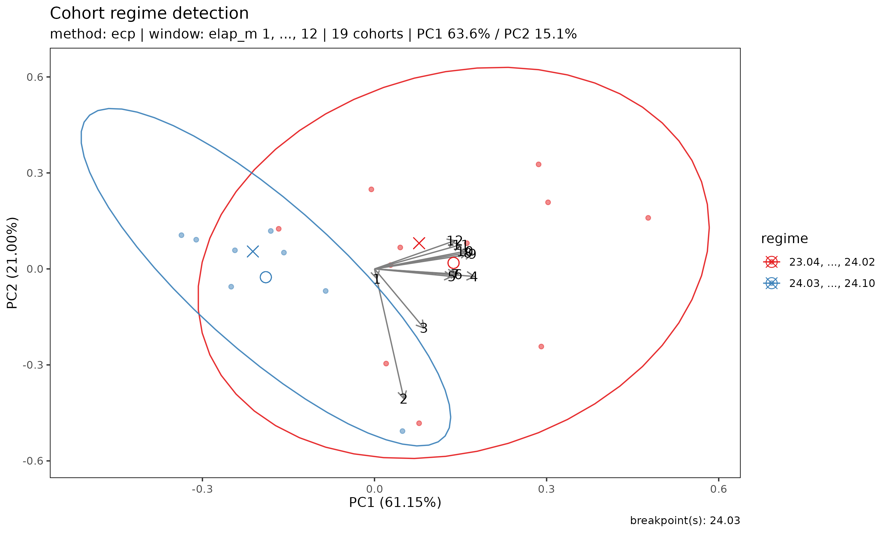

Arrows indicate the loadings of each development-period feature on the PC axes — useful for reading how the regimes differ (e.g. whether the shift primarily affects early or late development).

Choice of method

"ecp" — preferred default. Multivariate, non-parametric, auto-detects the number of regimes at a given significance level. Slightly slower than the alternatives but requires no a priori choice of n_regimes.
"pelt" — fast univariate change-point detection applied to the first principal component. May return multiple breakpoints and is useful when the trajectory variation is dominated by one axis (check PC1 % in the print() output — if > 70%, PELT is reliable; if much lower, prefer "ecp").
"hclust" — Ward hierarchical clustering on the scaled feature matrix, cut to n_regimes clusters (default 2). Ignores chronological order and is best used as a sanity check: if the chronological methods locate a breakpoint at time t and hclust produces the same two groups (all pre-t in one cluster, all post-t in the other), the shift is structural rather than an artefact of the method.

In practice, agreement across all three methods — as in the SUR example above, where "ecp", "pelt", and "hclust" all locate 24.04 as the regime boundary — is strong evidence of a real underwriting/rate shift.

Forcing the number of regimes

If you want to compare a fixed number of regimes — for example, two-vs-three regime hypotheses — pass n_regimes:

r2 <- detect_cohort_regime(tri_sur, K = 12, method = "ecp", n_regimes = 3)
summary(r2)
#> Cohort regime detection summary
#>   method    : ecp
#>   value_var : clr
#>   window    : elap_m 1, ..., 12
#>   cohorts   : 19 analysed (11 dropped)
#> 
#> Regimes (3):
#>   1: 23.04, ..., 23.06 (3 cohorts)
#>   2: 23.07, ..., 24.02 (8 cohorts)
#>   3: 24.03, ..., 24.10 (8 cohorts)
#> 
#> Breakpoints: 23.07, 24.03

For "ecp" and "pelt", n_regimes is a request (the algorithm will return up to that many regimes if supported by the data). For "hclust", it is a hard cut.

Relation to `fit_lr()`

detect_cohort_regime() is a preprocessing diagnostic, not a modification of the fit_lr() framework. Its output is useful in two ways:

Stratified fitting: if two clearly distinct regimes are detected, fitting fit_lr() separately on each regime subset often yields sharper stable-CLR estimates than a pooled fit.
Rate-change documentation: a detected breakpoint provides a data-driven anchor for the preprocessing recommendations outlined in the Limitations section of the companion paper (premium on-leveling or exposure decomposition V = C^P / r).