Aggregation frameworks: Triangle, Calendar, Total • lossratio

The same long-format experience data can be aggregated three ways depending on the question being asked. lossratio exposes one builder per framework. This vignette compares them.

At a glance

Builder	Output object	Dimension	When to use
`build_triangle()`	`Triangle`	cohort × dev (2D)	SA, ED, CL projection
`build_calendar()`	`Calendar`	calendar period (1D)	Calendar-year trend, diagonal effect
`build_total()`	`Total`	portfolio total (per group)	High-level loss-ratio comparison

Conceptually:

Triangle preserves both the cohort axis (when policies were underwritten) and the development axis (how loss accrues over development time). This is the canonical chain-ladder data structure.
Calendar collapses cohorts onto the diagonal — each row is one calendar period across all underwriting cohorts. Equivalent to the diagonal sum of the triangle.
Total collapses both dimensions to one value per group. Useful for portfolio-level comparison (which product had the worst loss ratio over the window?).

Triangle (cohort × dev)

library(lossratio)
data(experience)
exp <- as_experience(experience)

tri <- build_triangle(exp, group_var = cv_nm)
head(tri)
#>     cv_nm n_obs     cohort   dev   loss       rp  closs      crp   margin
#>    <char> <int>     <Date> <int>  <num>    <num>  <num>    <num>    <num>
#> 1:    SUR    30 2023-04-01     1      0 11191622      0 11191622 11191622
#> 2:    CAN    30 2023-04-01     1   6445 12879191   6445 12879191 12872746
#> 3:    2CI    30 2023-04-01     1 468845  7567723 468845  7567723  7098878
#> 4:    HOS    30 2023-04-01     1      0 15273272      0 15273272 15273272
#> 5:    SUR    29 2023-04-01     2      0 14025885      0 25217507 14025885
#> 6:    CAN    29 2023-04-01     2      0 30821344   6445 43700535 30821344
#>     cmargin profit cprofit           lr          clr  loss_prop   rp_prop
#>       <num> <fctr>  <fctr>        <num>        <num>      <num>     <num>
#> 1: 11191622    pos     pos 0.0000000000 0.0000000000 0.00000000 0.2385673
#> 2: 12872746    pos     pos 0.0005004196 0.0005004196 0.01356014 0.2745405
#> 3:  7098878    pos     pos 0.0619532454 0.0619532454 0.98643986 0.1613181
#> 4: 15273272    pos     pos 0.0000000000 0.0000000000 0.00000000 0.3255741
#> 5: 25217507    pos     pos 0.0000000000 0.0000000000 0.00000000 0.1890296
#> 6: 43694090    pos     pos 0.0000000000 0.0001474810 0.00000000 0.4153853
#>     closs_prop  crp_prop
#>          <num>     <num>
#> 1: 0.000000000 0.2385673
#> 2: 0.013560142 0.2745405
#> 3: 0.986439858 0.1613181
#> 4: 0.000000000 0.3255741
#> 5: 0.000000000 0.2082178
#> 6: 0.008953204 0.3608298

Each row is one (cohort, dev) cell with cumulative loss / risk premium. Visualise as line plot or heatmap:

plot(tri)              # one trajectory per cohort, faceted by group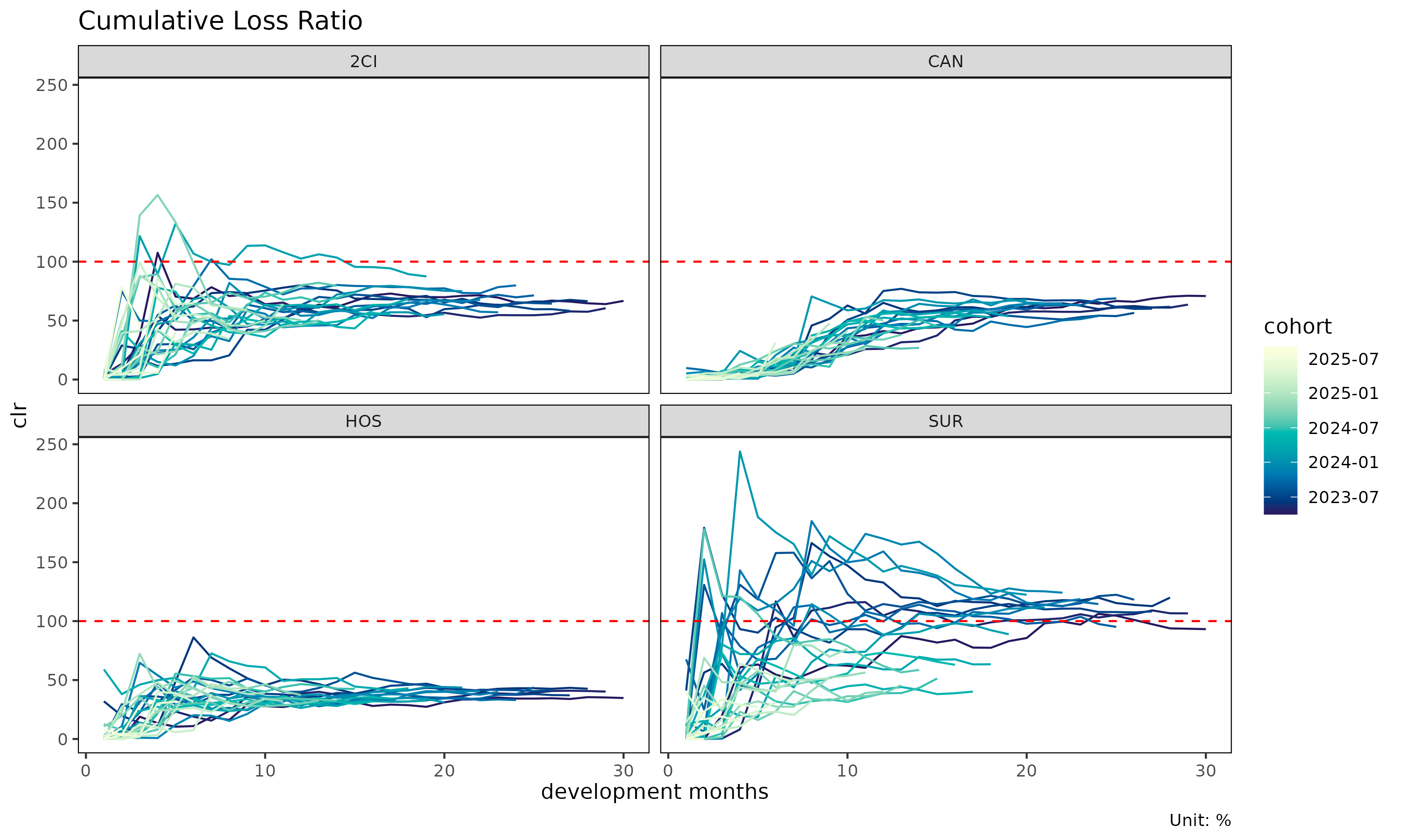


# With multiple group panels each panel's cells get too narrow to read,
# so use quarterly cohort and dev to bring each panel down to ~10 x 10
# cells. This fits the documentation's display size; in practice you
# can keep monthly resolution by enlarging the plot.
tri_q <- build_triangle(exp, group_var = cv_nm,
                        cohort_var = "uyq", dev_var = "elap_q")
plot_triangle(tri_q)   # cohort × dev heatmap of clr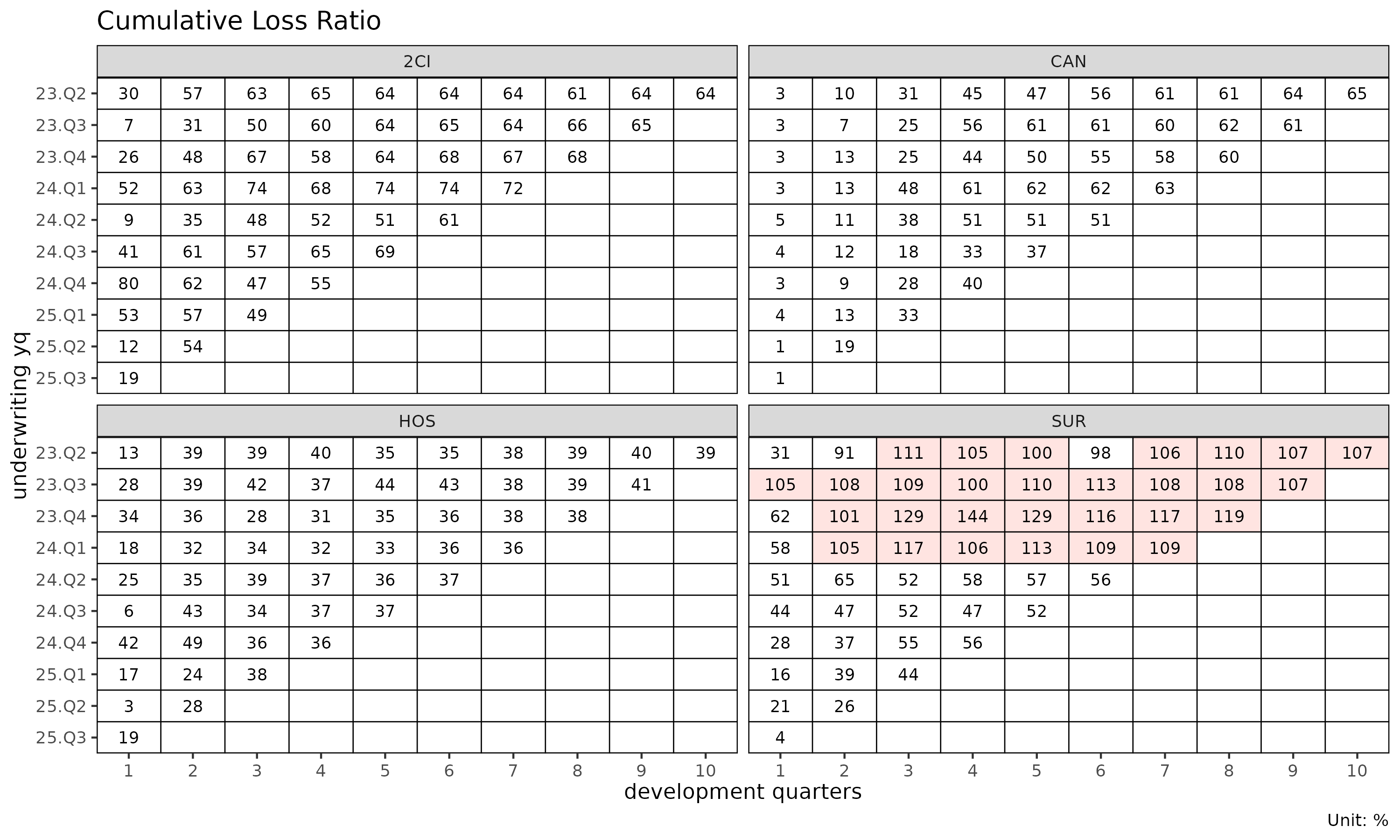

Use Triangle as input to: - build_ata(), build_ed() — development factors - fit_cl(), fit_lr() — projection - detect_cohort_regime() — structural change detection

Calendar (calendar period only)

cal <- build_calendar(exp, group_var = cv_nm, calendar_var = "cym")
head(cal)
#>     cv_nm   calendar   dev     loss        rp     closs       crp   margin
#>    <char>     <Date> <int>    <num>     <num>     <num>     <num>    <num>
#> 1:    2CI 2023-04-01     1   468845   7567723    468845   7567723  7098878
#> 2:    2CI 2023-05-01     2   788082  27286688   1256927  34854411 26498606
#> 3:    2CI 2023-06-01     3 18122450  42665533  19379377  77519944 24543083
#> 4:    2CI 2023-07-01     4 70259233  68265637  89638610 145785581 -1993596
#> 5:    2CI 2023-08-01     5 32739949 110351072 122378559 256136653 77611123
#> 6:    2CI 2023-09-01     6 61587160 135154735 183965719 391291388 73567575
#>      cmargin profit cprofit         lr        clr loss_prop   rp_prop
#>        <num> <fctr>  <fctr>      <num>      <num>     <num>     <num>
#> 1:   7098878    pos     pos 0.06195325 0.06195325 0.9864399 0.1613181
#> 2:  33597484    pos     pos 0.02888156 0.03606221 0.9626040 0.2248381
#> 3:  58140567    pos     pos 0.42475621 0.24999214 0.3480569 0.1688936
#> 4:  56146971    neg     pos 1.02920351 0.61486609 0.4423512 0.2060648
#> 5: 133758094    pos     pos 0.29668900 0.47778620 0.2173682 0.2219566
#> 6: 207325669    pos     pos 0.45567889 0.47015019 0.2061898 0.2113124
#>    closs_prop  crp_prop
#>         <num>     <num>
#> 1:  0.9864399 0.1613181
#> 2:  0.9713591 0.2071298
#> 3:  0.3631717 0.1841805
#> 4:  0.4224394 0.1938191
#> 5:  0.3373051 0.2050163
#> 6:  0.2781021 0.2071482

Each row is one calendar period (per group). The dev column here is a sequential index (1, 2, 3, …) within group, not “development period since cohort start”.

Calendar aggregation is mathematically the diagonal sum of the triangle: cells with the same cym (regardless of uym/elap_m) are combined.

Use cases: - Trend analysis (“loss ratio is rising over calendar time”) - Calendar-year effect detection (e.g., regulatory shock, premium on-leveling event) - Portfolio monitoring dashboards

plot(cal)                       # x axis: calendar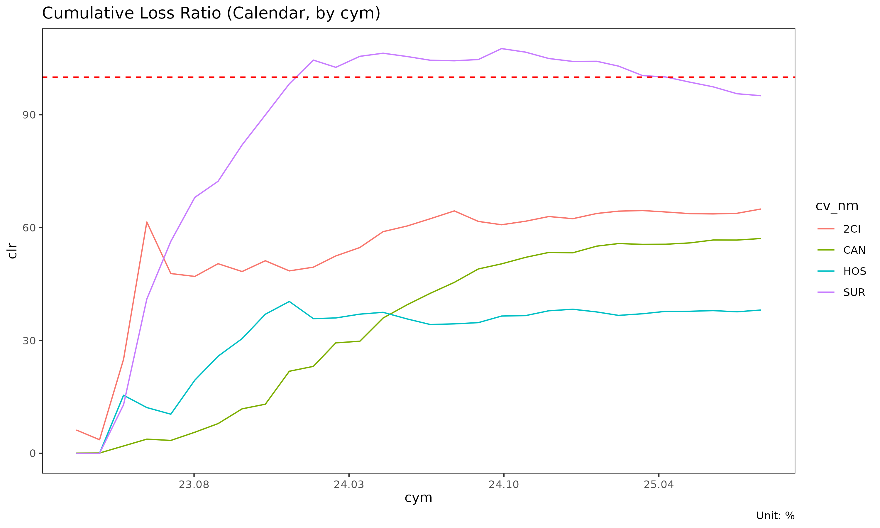

plot(cal, x_by = "dev")         # x axis: sequential index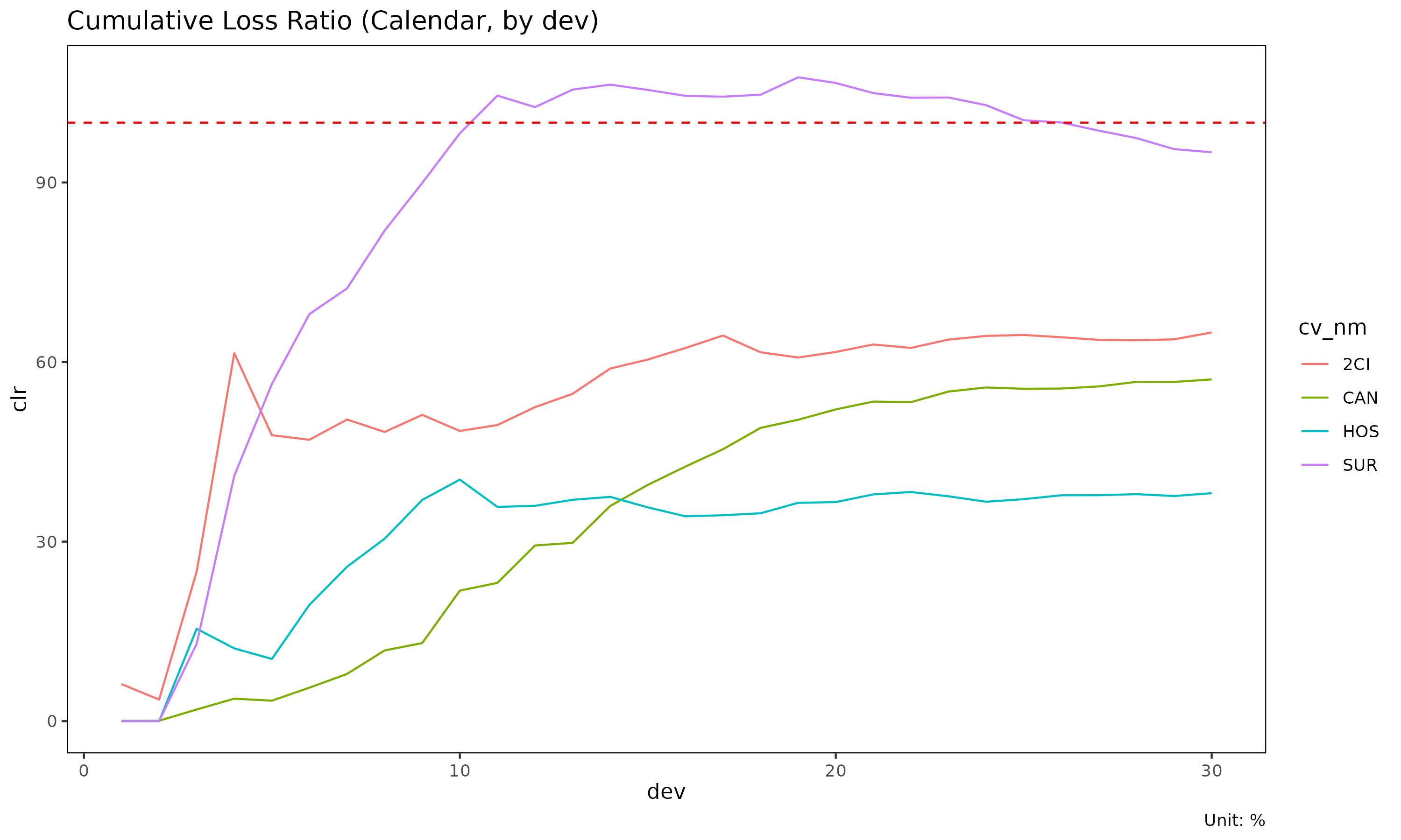

Total (portfolio summary)

tot <- build_total(
  exp,
  group_var = cv_nm,
  cohort_var = "uym",
  period_from = "2023-04-01",
  period_to   = "2024-03-01"
)
head(tot)
#>     cv_nm n_obs sales_start  sales_end        loss          rp        lr
#>    <char> <int>      <Date>     <Date>       <num>       <num>     <num>
#> 1:    SUR    30  2023-04-01 2024-03-01 26195800145 23817090339 1.0998741
#> 2:    CAN    30  2023-04-01 2024-03-01 15036650678 24008537158 0.6263043
#> 3:    2CI    30  2023-04-01 2024-03-01 12482828960 18720199627 0.6668107
#> 4:    HOS    30  2023-04-01 2024-03-01  9737095690 25111393787 0.3877561
#>    loss_prop   rp_prop
#>        <num>     <num>
#> 1: 0.4128419 0.2598496
#> 2: 0.2369754 0.2619383
#> 3: 0.1967275 0.2042414
#> 4: 0.1534552 0.2739707

One row per group, summarising loss / risk premium / loss ratio over the window. The period_from / period_to arguments restrict to a fixed window so groups are comparable.

Use cases: - Compare overall loss ratio across coverages - Rank groups by reserve / share of portfolio - Build executive summary tables

Aggregation as data flow

                     experience (long, with demographics)
                              │
         ┌────────────────────┼─────────────────────┐
         │                    │                     │
   build_triangle      build_calendar         build_total
   (cohort × dev)      (calendar series)     (portfolio total)
         │                    │                     │
         ▼                    ▼                     ▼
     Triangle             Calendar               Total
   (2D, projection)     (1D, trend)         (0D, comparison)

All three start from the same experience and aggregate demographic dimensions away. Choose the framework based on the analytical question.

Attribute schema

After aggregation, each object stores its source-column metadata as attributes (used for plot labels and granularity-aware date formatting):

attr(tri, "cohort_var")     # "uym"
#> [1] "uym"
attr(tri, "cohort_type")    # "month"
#> [1] "month"
attr(tri, "dev_var")        # "elap_m"
#> [1] "elap_m"
attr(tri, "dev_type")       # "month"
#> [1] NA

attr(cal, "calendar_var")   # "cym"
#> [1] "cym"
attr(cal, "calendar_type")  # "month"
#> [1] "month"

The data columns themselves are standardised to cohort / dev / calendar, so downstream code is granularity-agnostic.