Before fitting a chain ladder or loss-ratio model, it pays to inspect
the underlying triangle. This vignette covers the diagnostic tools in
lossratio for understanding cohort behaviour, age-to-age
factor stability, and maturity detection.
Triangle-level diagnostics
For brevity this vignette uses the SUR group only —
every step generalises to multi-group input.
library(lossratio)
data(experience)
exp <- as_experience(experience)[cv_nm == "SUR"]
tri <- build_triangle(exp, group_var = cv_nm)
Cohort trajectories
plot(tri) # raw clr trajectories per cohort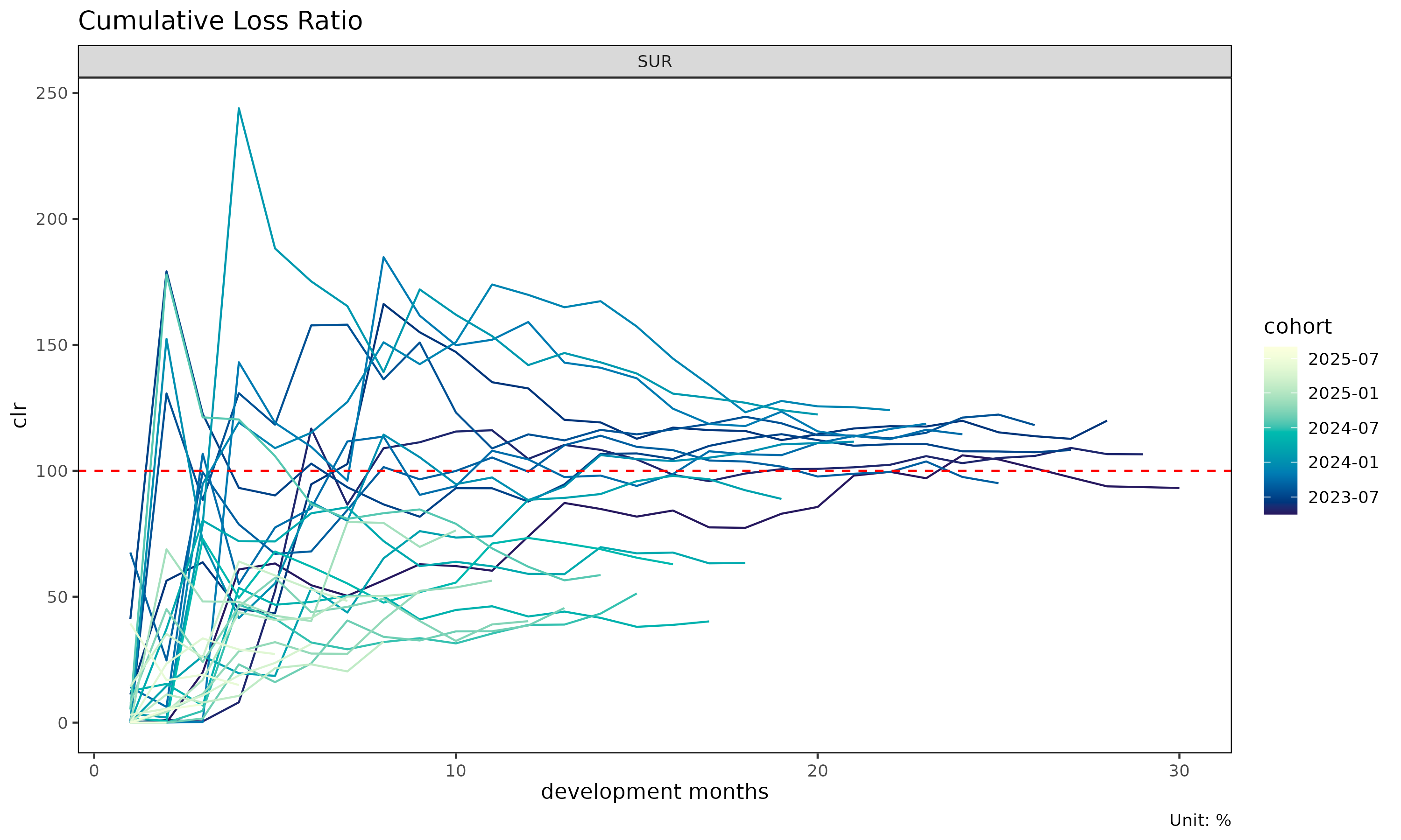
plot(tri, value_var = "lr") # incremental loss ratio instead of clr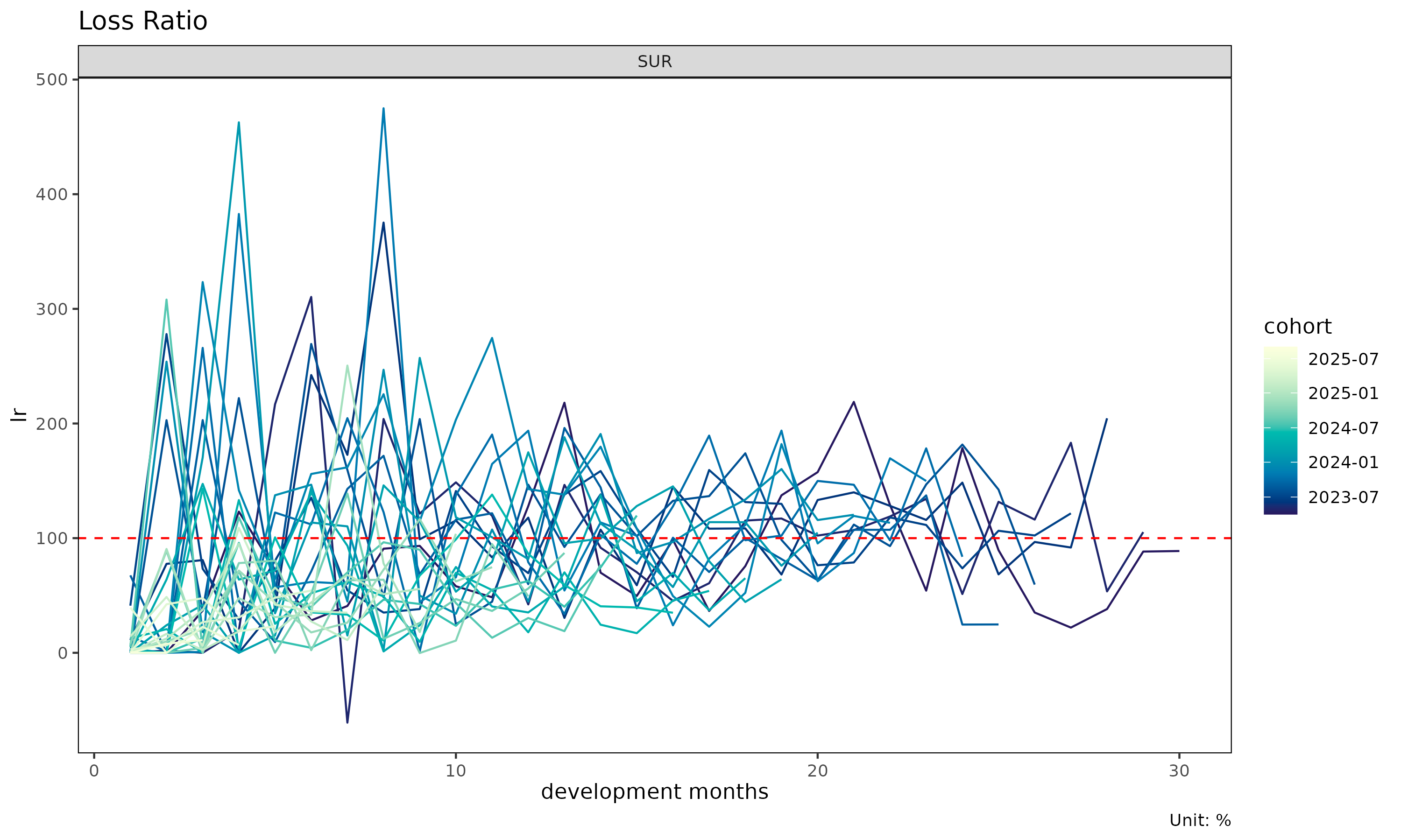
plot(tri, summary = TRUE) # raw + overlay (mean / median / weighted)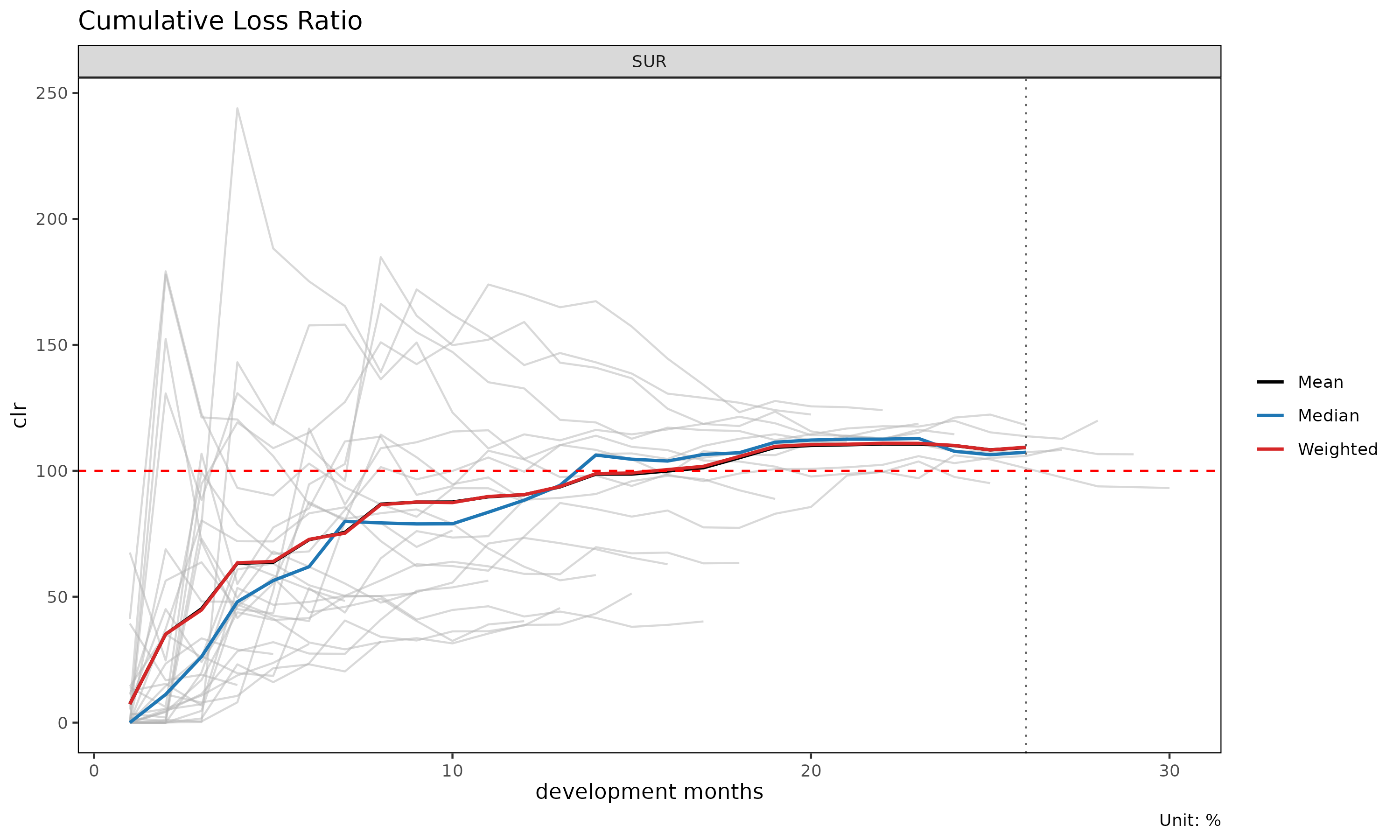
The summary = TRUE overlay computes mean, median, and
weighted clr at each dev and overlays them on the cohort lines. Useful
for spotting cohorts that deviate from the central tendency.
Cell heatmap
plot_triangle(tri) # clr in each cell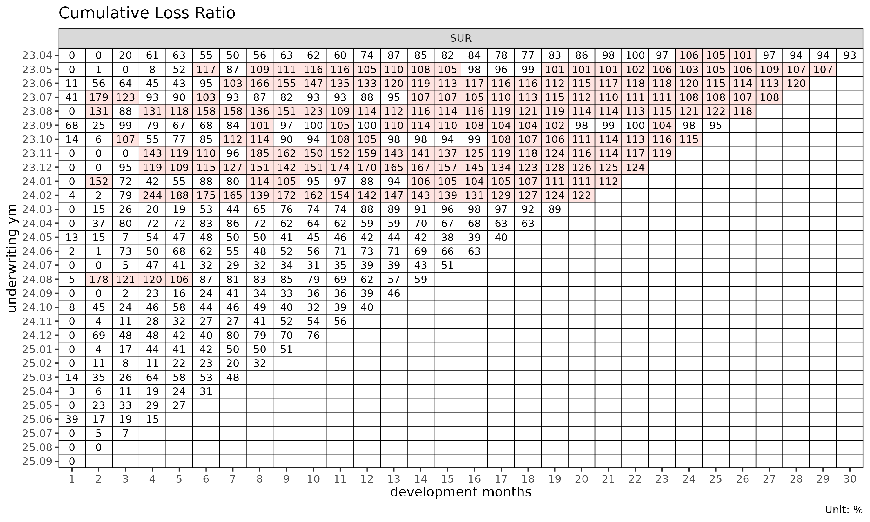
plot_triangle(tri, value_var = "lr") # incremental loss ratio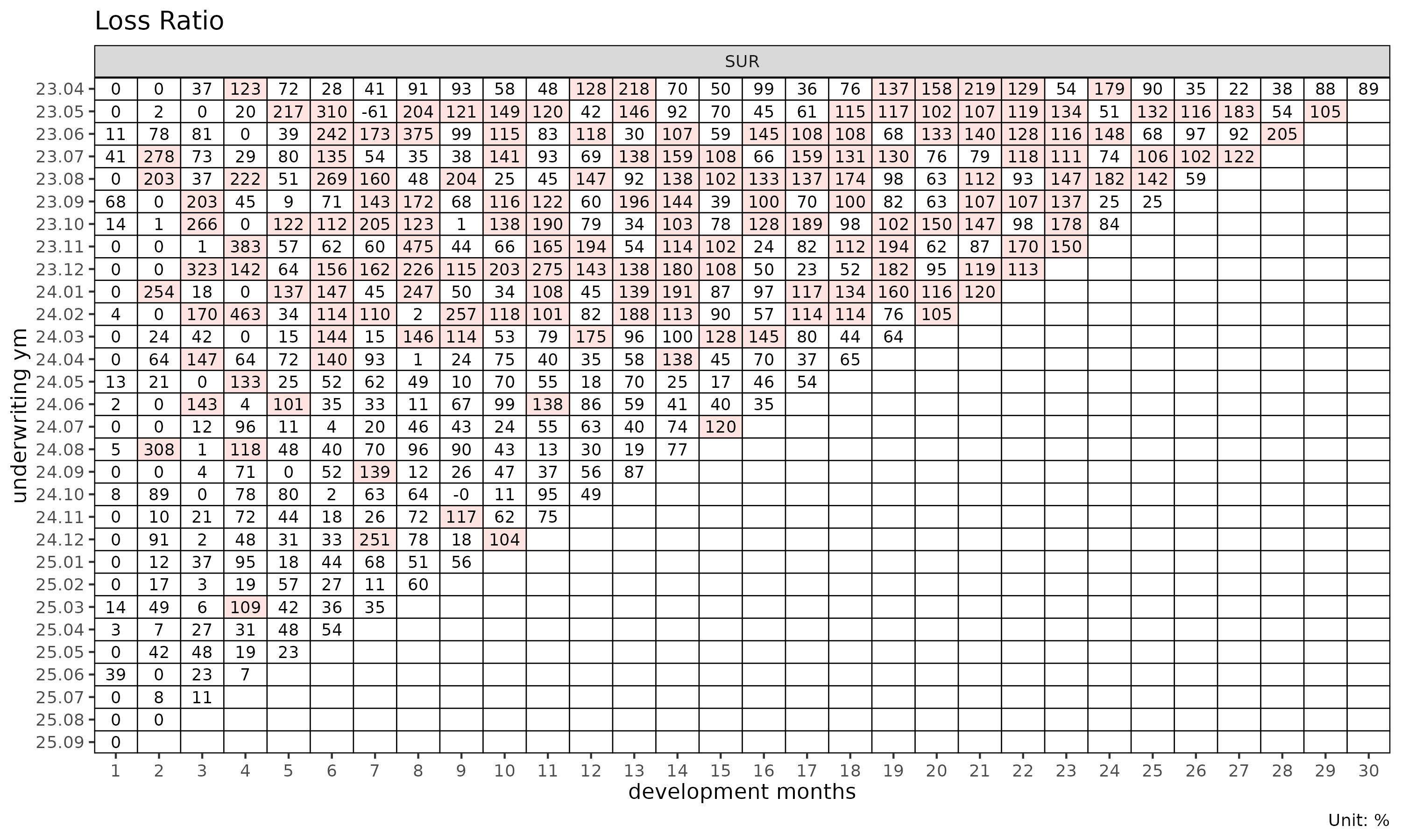
# detail labels (ratio + loss/rp amounts) are 2-line — use quarterly cells
tri_q <- build_triangle(exp, group_var = cv_nm,
                        cohort_var = "uyq", dev_var = "elap_q")
plot_triangle(tri_q, label_style = "detail")  # ratio + (loss / rp) amounts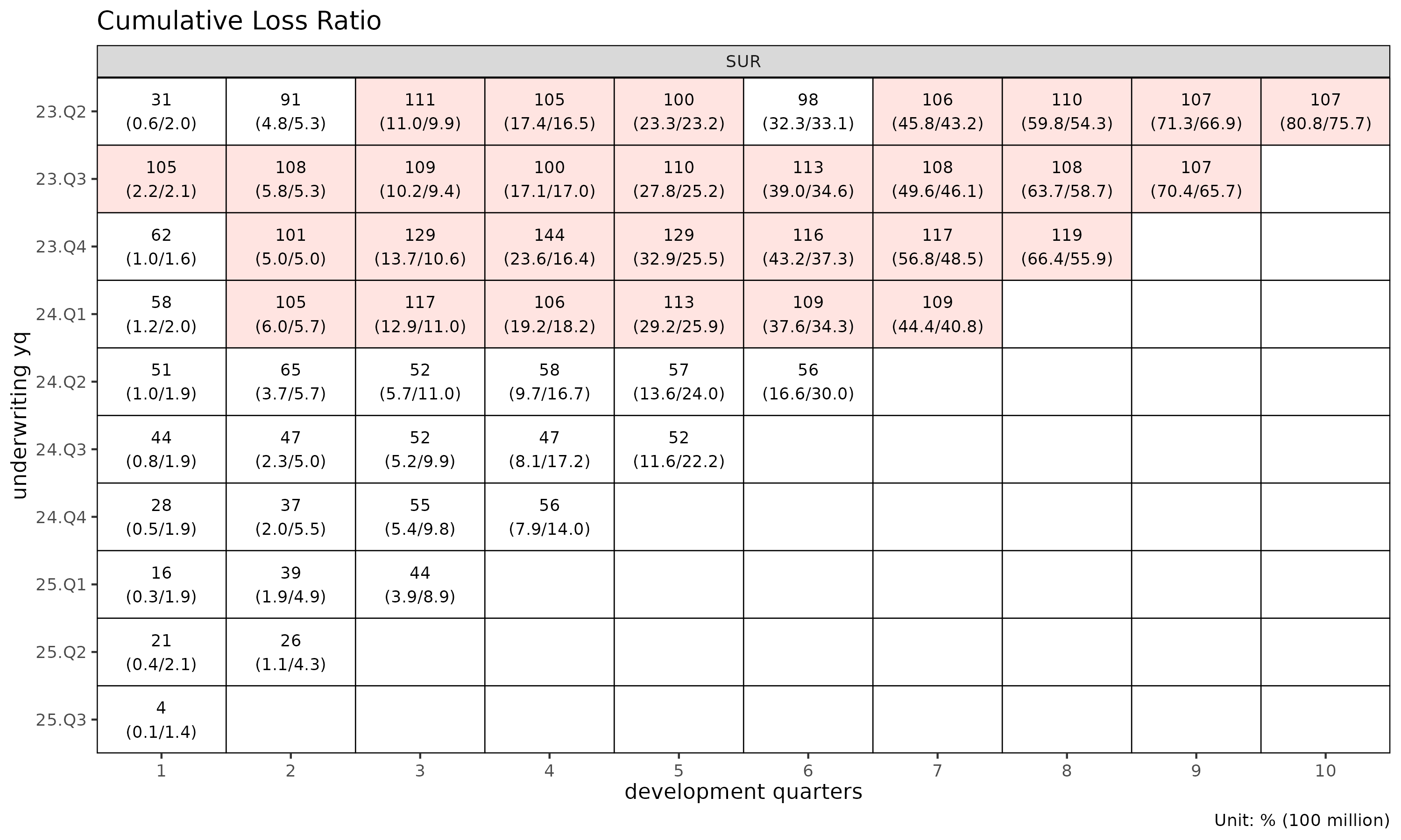
Group statistics by dev
sm <- summary(tri)
head(sm)
#> Key: <cv_nm, dev>
#>     cv_nm   dev n_obs   lr_mean lr_median      lr_wt  clr_mean clr_median
#>    <char> <int> <int>     <num>     <num>      <num>     <num>      <num>
#> 1:    SUR     1    30 0.0738546 0.0000000 0.07343113 0.0738546  0.0000000
#> 2:    SUR     2    29 0.5365888 0.0992849 0.54126362 0.3512535  0.1120447
#> 3:    SUR     3    28 0.6201189 0.2472070 0.56590118 0.4521326  0.2618096
#> 4:    SUR     4    27 0.8852657 0.6387164 0.92060611 0.6327242  0.4798531
#> 5:    SUR     5    26 0.5767556 0.4828899 0.59880663 0.6369307  0.5641166
#> 6:    SUR     6    25 0.9314593 0.5431397 0.95085711 0.7264308  0.6191132
#>        clr_wt
#>         <num>
#> 1: 0.07343113
#> 2: 0.35150128
#> 3: 0.44744109
#> 4: 0.63467048
#> 5: 0.63999290
#> 6: 0.72781355
Returns a TriangleSummary object with mean / median /
weighted loss ratios per (group, dev) cell.
Age-to-age factor diagnostics
ata <- build_ata(tri, value_var = "closs")
sm  <- summary(ata, alpha = 1)
head(sm)
#> Key: <cv_nm>
#>     cv_nm ata_from ata_to ata_link   mean median     wt    cv     f  f_se   rse
#>    <char>    <num>  <num>   <fctr>  <num>  <num>  <num> <num> <num> <num> <num>
#> 1:    SUR        1      2      1-2 60.965  4.062 11.320 3.111 6.768 4.767 0.704
#> 2:    SUR        2      3      2-3 15.316  2.005  2.083 2.955 1.939 1.284 0.663
#> 3:    SUR        3      4      3-4 36.458  2.167  2.167 4.493 2.167 2.434 1.123
#> 4:    SUR        4      5      4-5  1.641  1.282  1.291 0.854 1.291 0.115 0.089
#> 5:    SUR        5      6      5-6  1.607  1.334  1.461 0.455 1.461 0.113 0.078
#> 6:    SUR        6      7      6-7  1.348  1.208  1.282 0.256 1.282 0.058 0.046
#>        sigma n_obs n_valid n_inf n_nan valid_ratio
#>        <num> <num>   <num> <num> <num>       <num>
#> 1: 27972.257    29      14     0     0       0.483
#> 2: 25358.337    28      24     0     0       0.857
#> 3: 69089.724    27      27     0     0       1.000
#> 4:  4787.739    26      26     0     0       1.000
#> 5:  5301.574    25      25     0     0       1.000
#> 6:  3279.239    24      24     0     0       1.000
The summary() method on an ATA object
computes per-link statistics that drive maturity detection:
-
mean,median,wt— descriptive averages of observed ata factors at each link (excluding cohorts where the link is not observed). -
cv— coefficient of variation of the observed factors (relative spread, alpha-independent). -
f— WLS-estimated factor (volume-weighted byvalue_from^alpha). -
f_se,rse— WLS standard error and relative standard error. -
sigma— Mack residual sigma per link. -
n_obs,n_valid,n_inf,n_nan,valid_ratio— observation counts and the share of finite ATA factors per link.
Diagnostic plots for ATA
plot(ata, type = "cv") # CV vs ata link with maturity overlay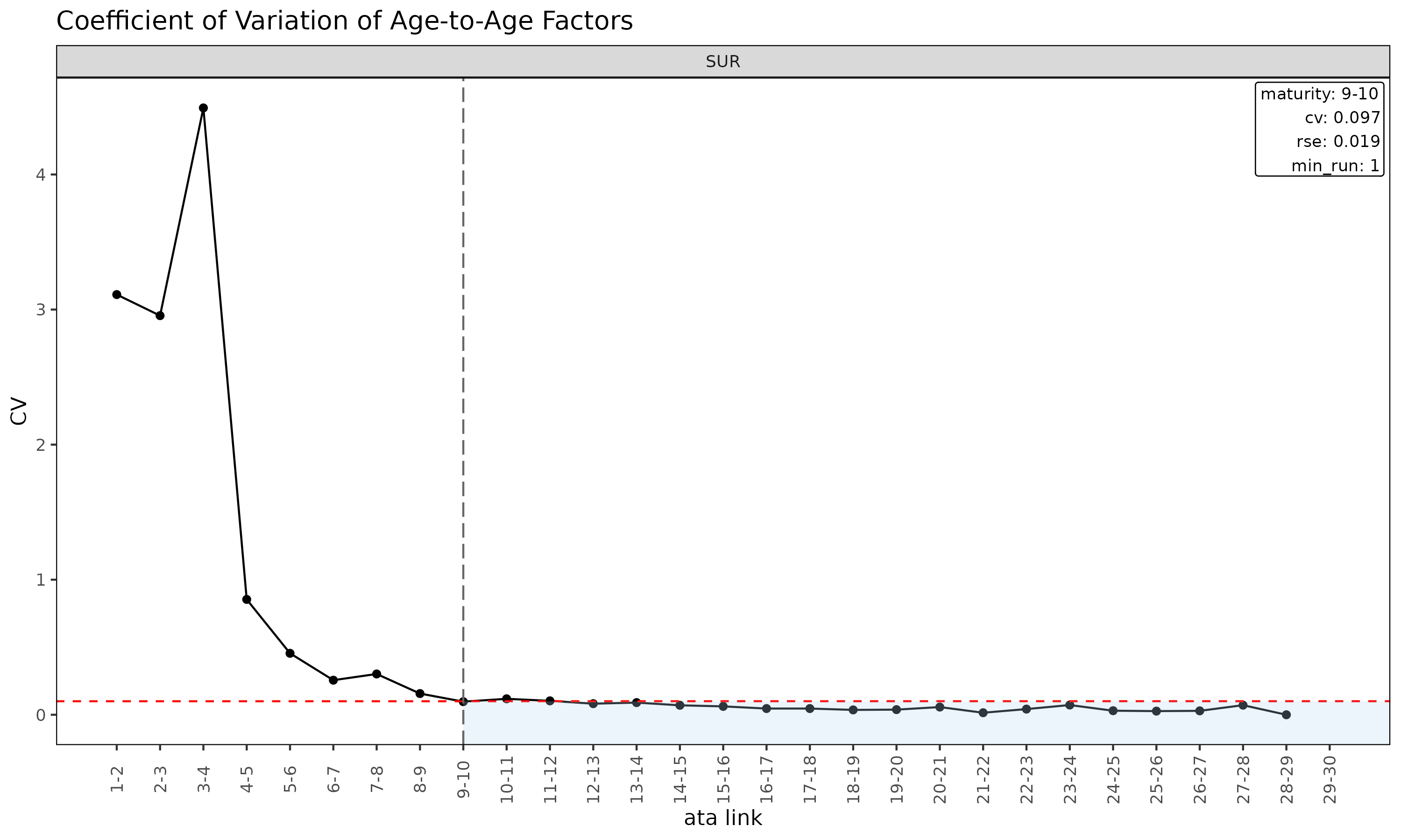
plot(ata, type = "rse") # RSE vs ata link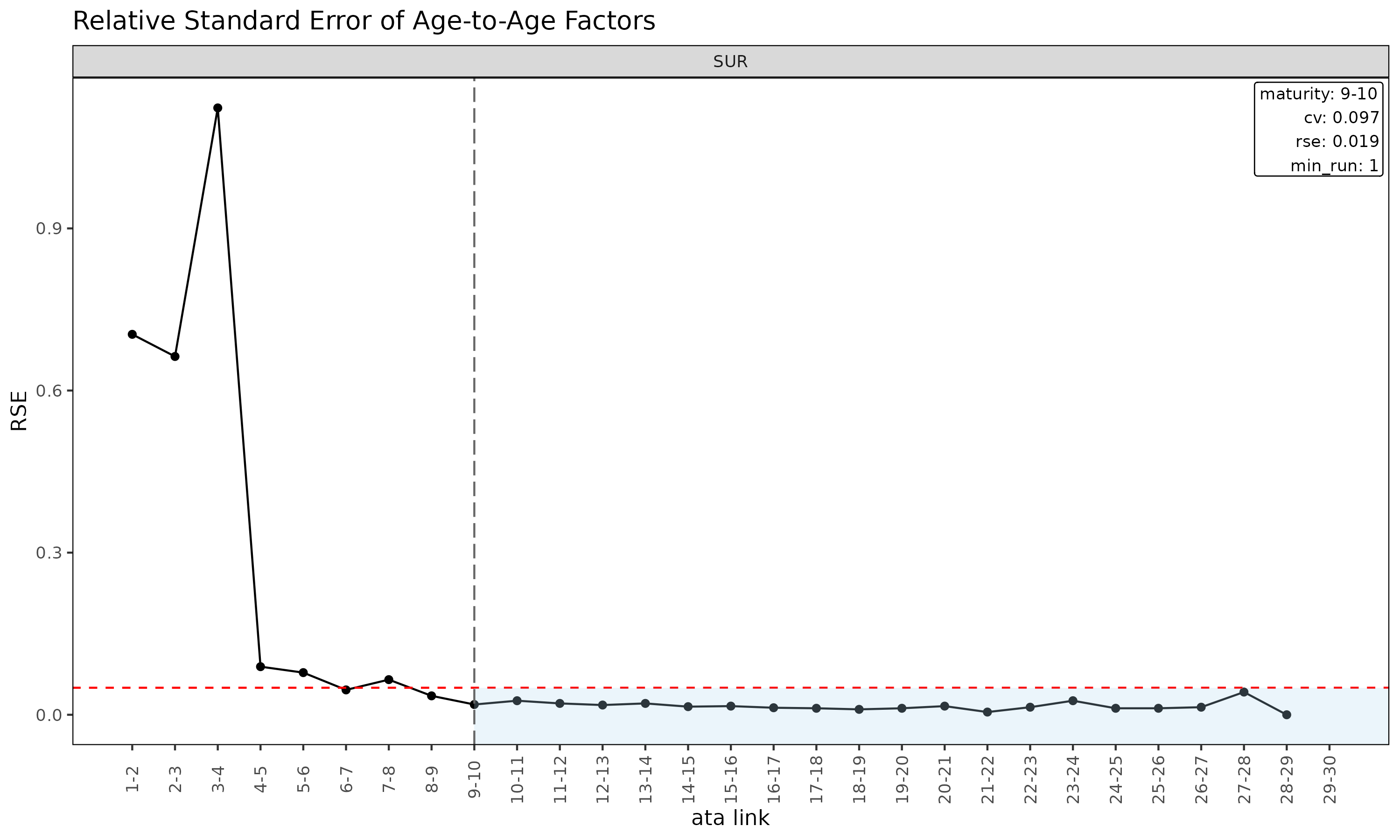
plot(ata, type = "summary") # mean / median / wt overlay per link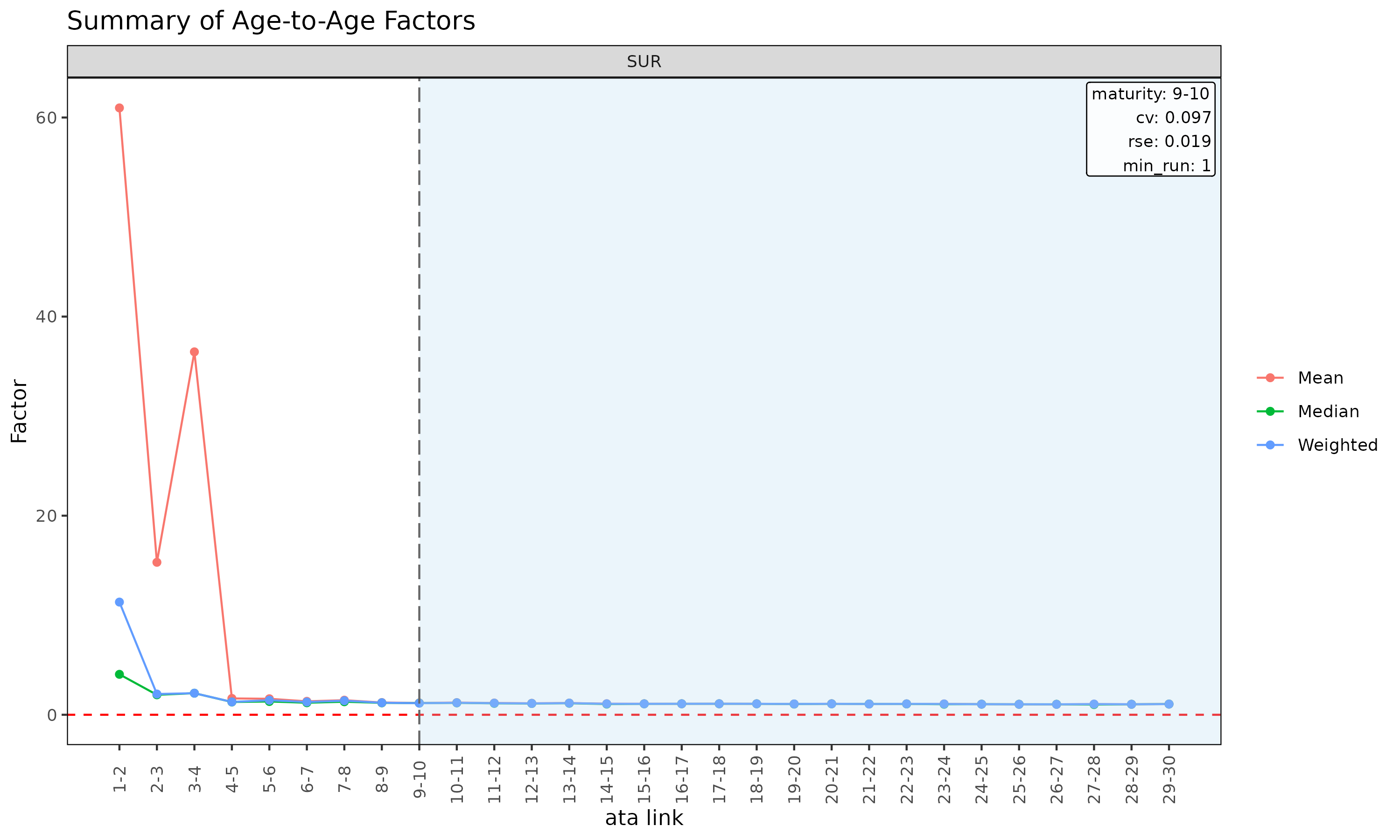
plot(ata, type = "box") # boxplot of observed ata per link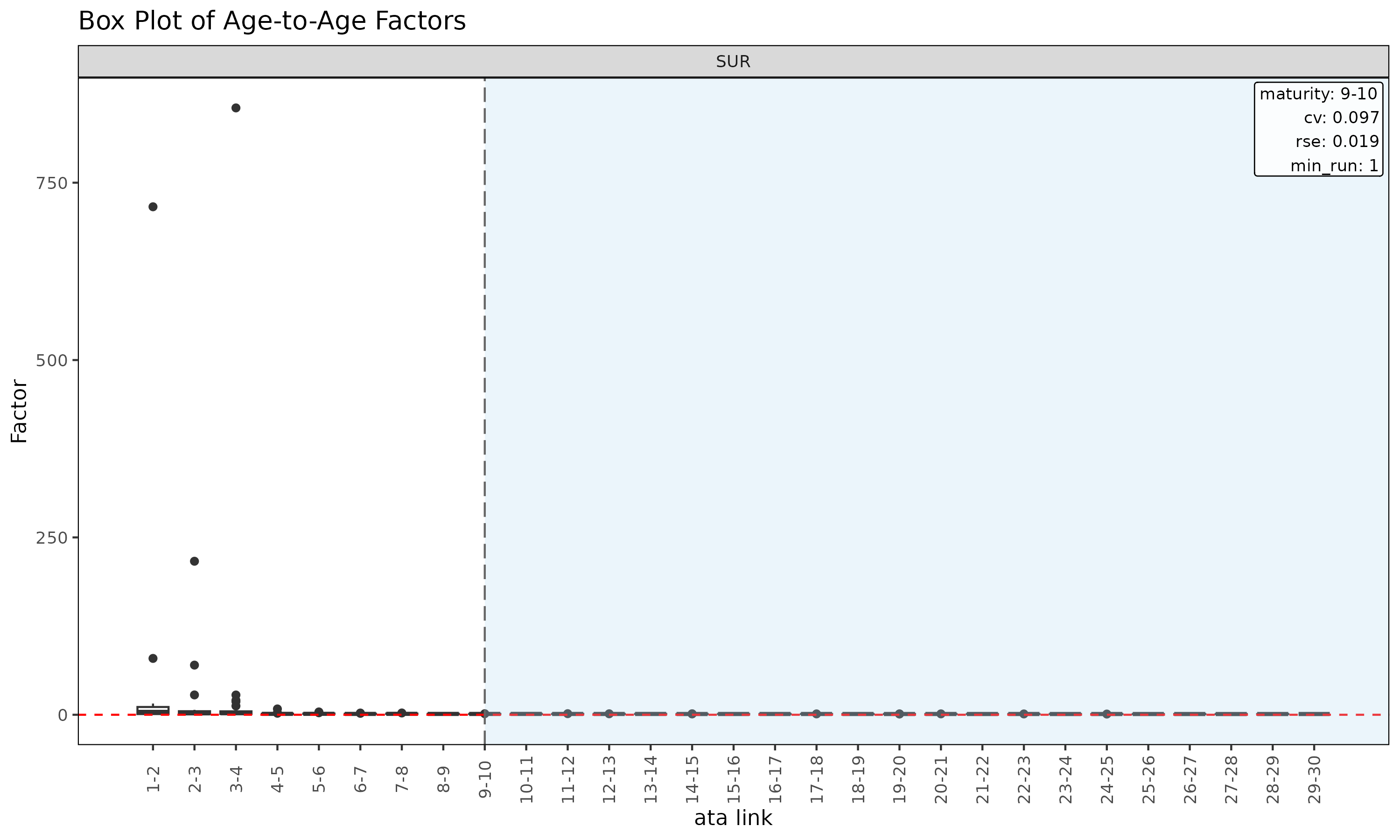
plot(ata, type = "point") # scatter of observed ata per link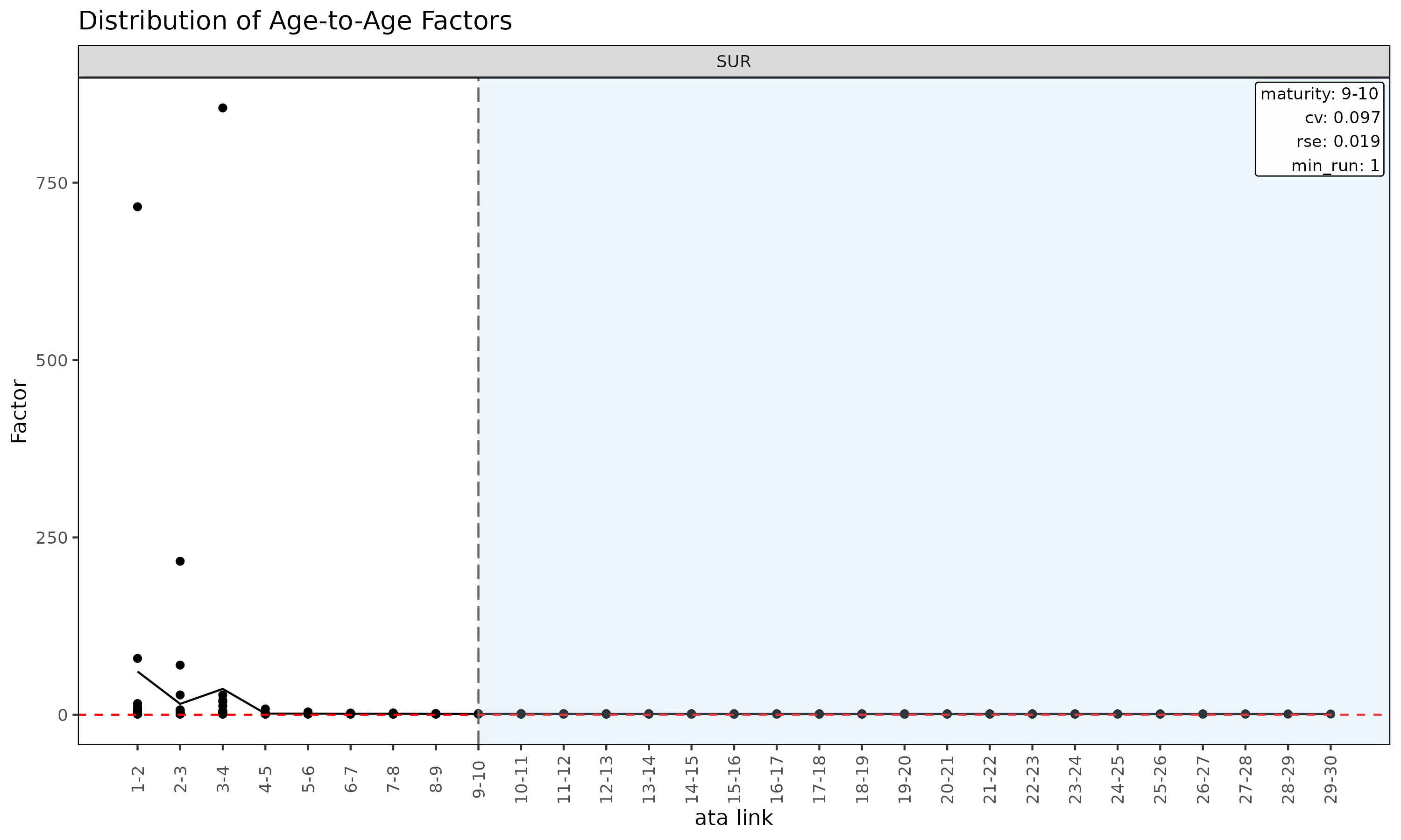
Triangle of ATA factors
la <- list(size = 2.5)                            # shrink labels
plot_triangle(ata, label_args = la)               # heatmap of observed factors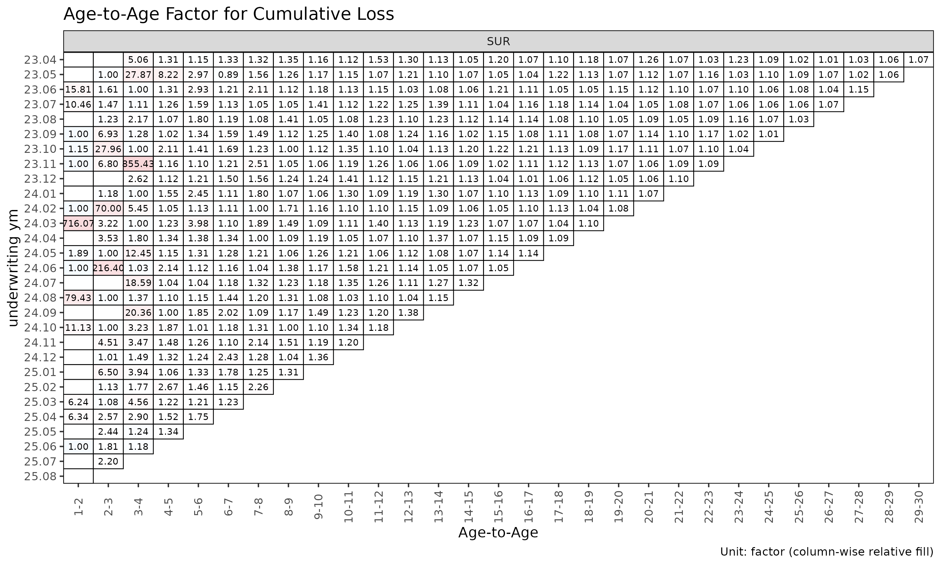
plot_triangle(ata, label_args = la, show_maturity = TRUE) # overlay maturity line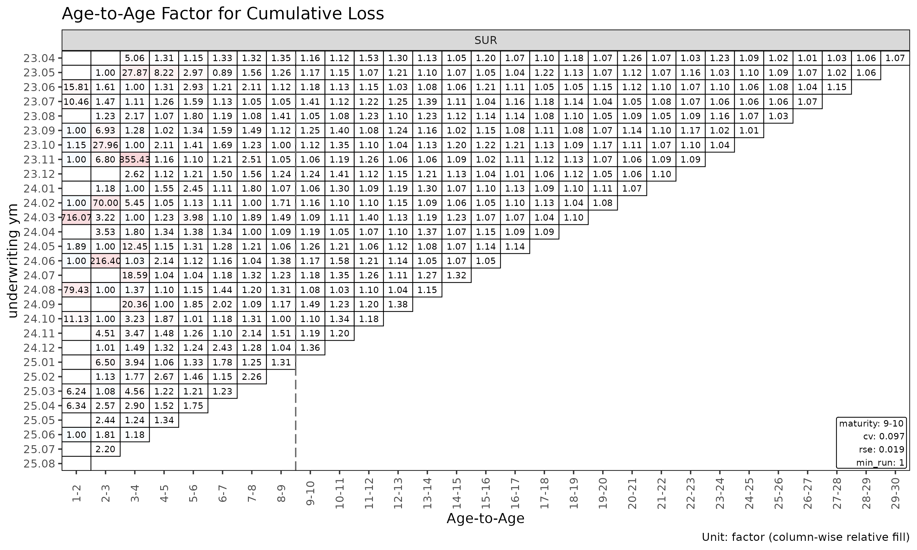
# detail labels are two lines and overlap on monthly cells — rebuild on the
# quarterly triangle so the labels fit
ata_q <- build_ata(tri_q, value_var = "closs")
plot_triangle(ata_q, label_style = "detail")      # factor + (loss / rp) amounts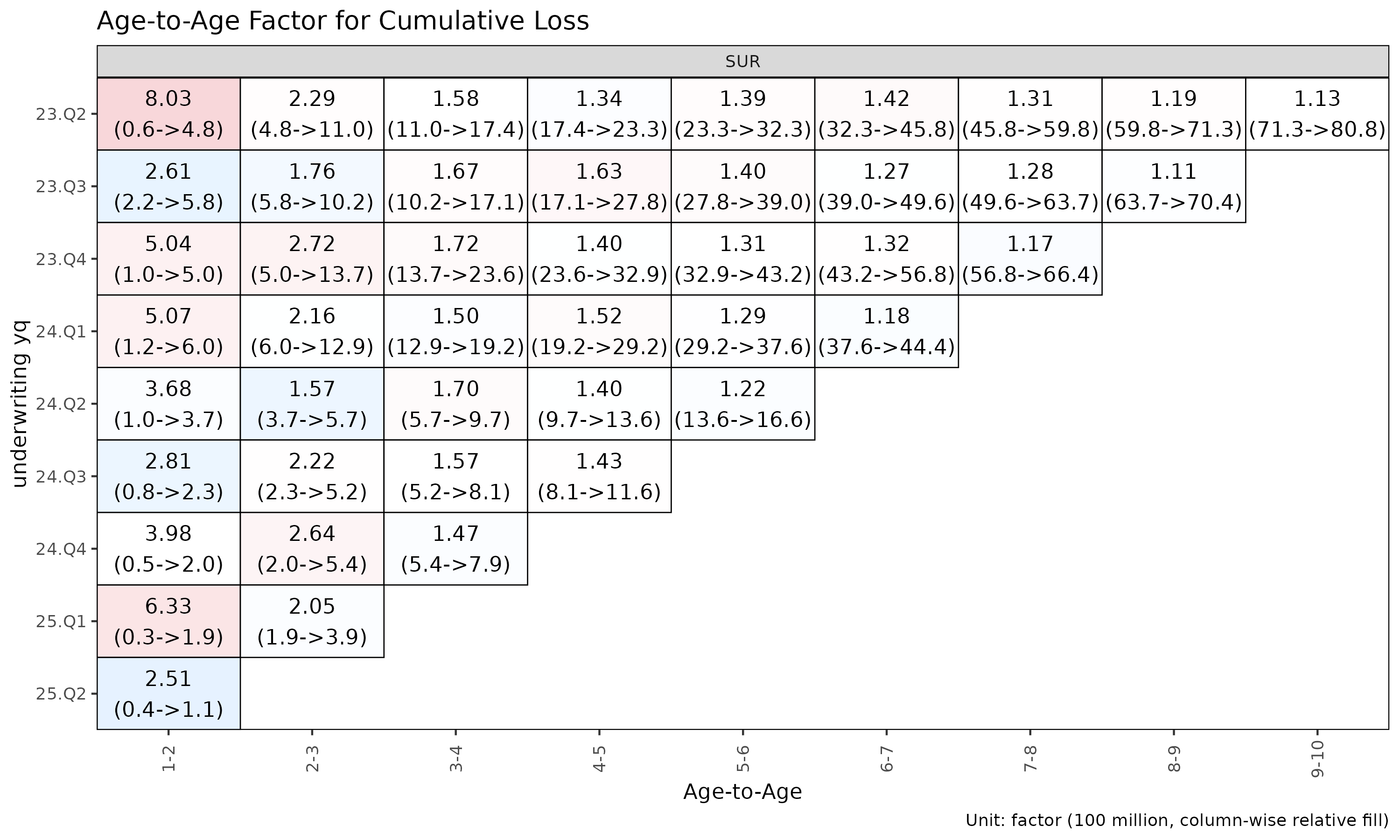
The heatmap colours each cell by log(ata / median(ata))
within its link, so column-wise colour distinguishes cohorts that
deviate from the link’s median.
Maturity detection
The maturity point is the development link beyond which age-to-age
factors are stable enough to trust for chain-ladder projection. Used
internally by fit_lr(method = "sa") to switch from ED to
CL.
find_ata_maturity() operates on a summary of an
ATA object — first build the descriptive / WLS summary via
summary(), then probe it for the first mature link:
sm  <- summary(ata, alpha = 1)
mat <- find_ata_maturity(
  sm,
  cv_threshold    = 0.10,    # CV must be below this
  rse_threshold   = 0.05,    # RSE must be below this
  min_valid_ratio = 0.5,     # at least 50% finite cohorts at the link
  min_n_valid     = 3L,      # at least 3 finite cohorts
  min_run         = 1L       # at least 1 consecutive mature link
)

print(mat)
#> Key: <cv_nm>
#>     cv_nm ata_from ata_to ata_link  mean median    wt    cv     f  f_se   rse
#>    <char>    <num>  <num>   <char> <num>  <num> <num> <num> <num> <num> <num>
#> 1:    SUR        9     10     9-10 1.188  1.172 1.165 0.097 1.165 0.022 0.019
#>       sigma n_obs n_valid n_inf n_nan valid_ratio
#>       <num> <num>   <num> <num> <num>       <num>
#> 1: 1774.278    21      21     0     0           1
A row per group with the first development link satisfying all
thresholds, carrying the link’s full statistics. The threshold arguments
are also stored as attributes on the returned object.
find_ata_maturity() is also called internally by
fit_ata() and fit_cl() when
maturity_args is supplied (the alpha of the
internal summary() step is taken from those callers).
Tune the thresholds to your portfolio’s volatility profile. Tight
thresholds (e.g. cv_threshold = 0.05) push maturity later;
loose thresholds push it earlier.
ED diagnostics
ed <- build_ed(tri, loss_var = "closs", exposure_var = "crp")
sm <- summary(ed, alpha = 1)
head(sm)
#> Key: <cv_nm>
#>     cv_nm ata_from ata_to ata_link    mean  median      wt      cv       g
#>    <char>    <num>  <num>   <fctr>   <num>   <num>   <num>   <num>   <num>
#> 1:    SUR        1      2      1-2 0.83638 0.11124 0.78549 1.64664 0.78549
#> 2:    SUR        2      3      2-3 0.42921 0.19355 0.39517 1.28530 0.39517
#> 3:    SUR        3      4      3-4 0.57740 0.28022 0.54349 1.36754 0.54349
#> 4:    SUR        4      5      4-5 0.18873 0.13962 0.18976 0.90510 0.18976
#> 5:    SUR        5      6      5-6 0.29944 0.16294 0.30277 1.01004 0.30277
#> 6:    SUR        6      7      6-7 0.21583 0.18880 0.20988 0.85987 0.20988
#>       g_se     rse    sigma n_obs n_valid n_inf n_nan valid_ratio
#>      <num>   <num>    <num> <num>   <num> <num> <num>       <num>
#> 1: 0.24877 0.31671 5291.085    29      29     0     0           1
#> 2: 0.09984 0.25264 3263.751    28      28     0     0           1
#> 3: 0.14933 0.27477 6210.872    27      27     0     0           1
#> 4: 0.03343 0.17615 1720.934    26      26     0     0           1
#> 5: 0.06037 0.19939 3487.836    25      25     0     0           1
#> 6: 0.03771 0.17970 2450.547    24      24     0     0           1

plot(ed, type = "summary")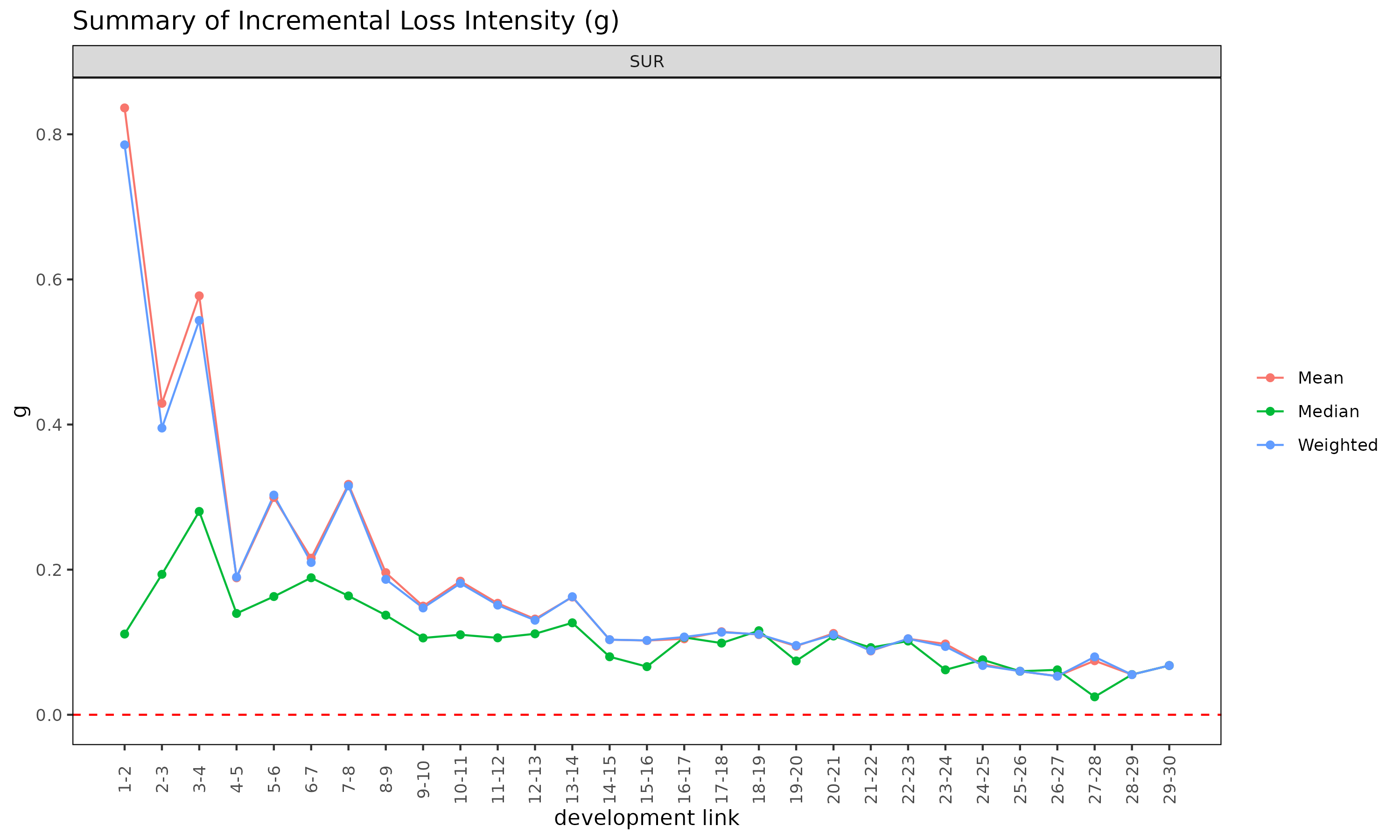
plot(ed, type = "box")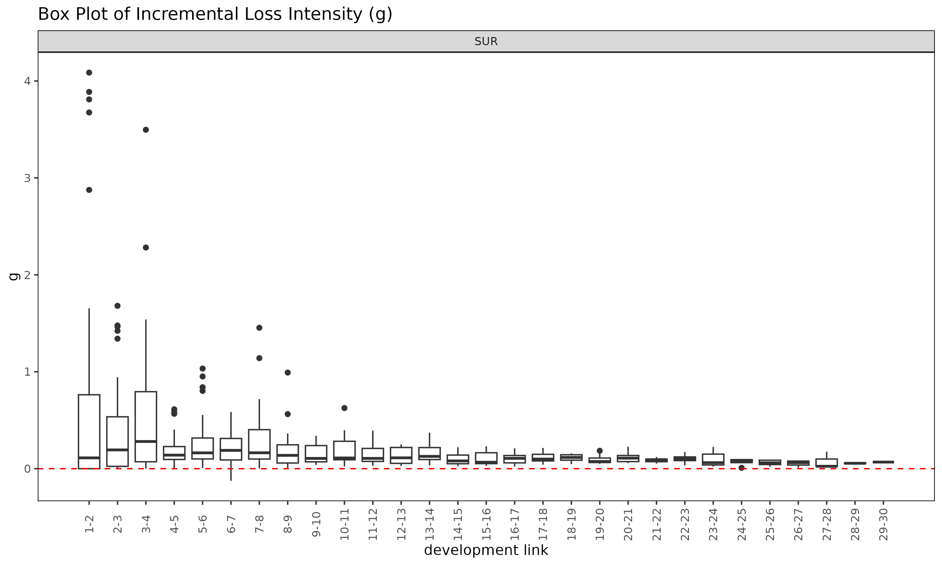
plot_triangle(ed, label_args = la)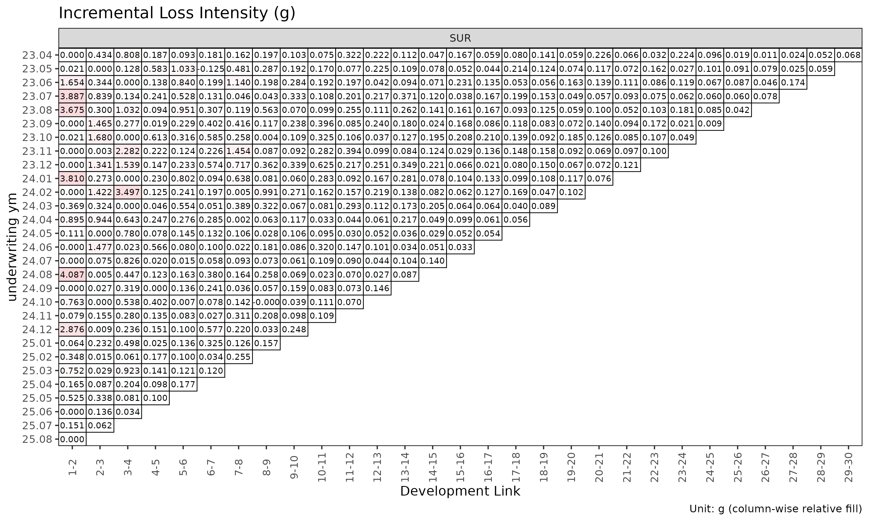
The summary() method on an ED object is the
ED-side analogue of summary() on an ATA
object, computing per-link statistics for the intensity
.
Validation before building
If gaps in the development sequence are suspected, inspect them
before build_triangle():
gaps <- validate_triangle(exp, group_var = cv_nm,
                          cohort_var = "uym", dev_var = "elap_m")
head(gaps)
#> Empty data.table (0 rows and 5 cols): cv_nm,uym,n_observed,n_expected,missing
Returns a TriangleValidation object with one row per
cohort that has non-consecutive development periods. An empty result
means the triangle is clean.
If gaps exist, options:
- Fix the data source (preferred).
- Drop offending cohorts.
- Pass
fill_gaps = TRUEtobuild_triangle()to zero-fill missing cells (use with care — inflatesn_obs).
Recent-diagonal subset
When older cohorts are no longer representative (rate change, reserving regime shift), restrict estimation to the recent calendar diagonals:
fit_ata(ata, alpha = 1, recent = 12)        # last 12 calendar diagonals
#> <ATAFit>
#> alpha       : 1
#> sigma_method: min_last2
#> recent      : 12
#> regime_break: none
#> use_maturity: FALSE
#> groups      : cv_nm
#> n_groups    : 1
#> ata links   : 29
fit_cl(tri, value_var = "closs", recent = 12)
#> <CLFit>
#> method      : basic
#> value_var   : closs
#> weight_var  : none
#> alpha       : 1
#> recent      : 12
#> use_maturity: FALSE
#> tail_factor : 1
#> groups      : cv_nm
#> periods     : 30
fit_lr(tri, recent = 12)
#> <LRFit>
#> method        : sa
#> loss_var      : closs
#> exposure_var  : crp
#> loss_alpha    : 1
#> exposure_alpha: 1
#> delta_method  : simple
#> conf_level    : 0.95
#> ci_type       : analytical
#> sigma_method  : min_last2
#> recent        : 12
#> regime_break  : none
#> maturity[SUR] : 18
#> groups        : cv_nm
#> periods       : 30
recent = K keeps only rows whose calendar position
(rank(cohort) + dev - 1) is among the latest K
per group.
Workflow checklist
Before fitting:
-
validate_triangle()— schema and gap check. -
build_triangle()— canonical shape with derived columns. -
plot(tri)/plot_triangle(tri)— visual inspection. -
summary(tri)— group-level central tendency. -
build_ata()+plot(ata, type = "cv")— link stability. -
find_ata_maturity()— verify maturity detection produces a sensible point per group. -
detect_cohort_regime()(optional) — structural change diagnosis.
Then fit fit_lr() / fit_cl() with
confidence in the input data.
See also
-
vignette("getting-started")— full pipeline overview. -
vignette("regime-detection")—detect_cohort_regime()deep dive. -
vignette("loss-ratio-methods")— projection method choice.