
This vignette walks the core functions of the lossratio package end to end, in the order prepare the data -> fit -> diagnose -> validate -> visualise. At each step it explains what is being called, why it behaves the way it does, and how to read the result. Reading this one document is enough to grasp the full workflow.
The problem this package solves
In long-term health insurance a policy, once underwritten, stays in force for decades. The central task is therefore to look ahead and see how a group of contracts written at a given point in time (a cohort) accumulates its loss ratio as the years pass.
lossratio frames this problem on a cohort x development-period (cohort x dev) grid.
- cohort – the time a contract was underwritten (e.g. January 2023 business).
- development period (dev) – the time elapsed since underwriting.
Each cell holds a cumulative loss (loss) and a
cumulative premium (premium), and the loss ratio is defined
as ratio = loss / premium. Estimating the cells of future
development periods that have not yet been observed is the act of
projection, and the various fit_* functions in this package
perform that estimate in different ways.
The data: experience
The package ships with a synthetic experience dataset. The term experience is the domain standard, referring to the cell-level records of an actuarial experience study.
data(experience)
str(experience)
#> Classes 'data.table' and 'data.frame':   2664 obs. of  15 variables:
#>  $ coverage    : chr  "ci" "ci" "ci" "ci" ...
#>  $ uy          : Date, format: "2023-01-01" "2023-01-01" ...
#>  $ uy_h        : Date, format: "2023-01-01" "2023-01-01" ...
#>  $ uy_q        : Date, format: "2023-01-01" "2023-01-01" ...
#>  $ uy_m        : Date, format: "2023-01-01" "2023-01-01" ...
#>  $ cy          : Date, format: "2023-01-01" "2023-01-01" ...
#>  $ cy_h        : Date, format: "2023-01-01" "2023-01-01" ...
#>  $ cy_q        : Date, format: "2023-01-01" "2023-01-01" ...
#>  $ cy_m        : Date, format: "2023-01-01" "2023-02-01" ...
#>  $ dev_y       : int  1 1 1 1 1 1 1 1 1 1 ...
#>  $ dev_h       : int  1 1 1 1 1 1 2 2 2 2 ...
#>  $ dev_q       : int  1 1 1 2 2 2 3 3 3 4 ...
#>  $ dev_m       : int  1 2 3 4 5 6 7 8 9 10 ...
#>  $ incr_loss   : num  1262380 11255763 11281309 33602387 7152622 ...
#>  $ incr_premium: num  27993106 29183931 29401966 26570540 27471886 ...
#>  - attr(*, ".internal.selfref")=<pointer: (nil)>
head(experience)
#>    coverage         uy       uy_h       uy_q       uy_m         cy       cy_h
#>      <char>     <Date>     <Date>     <Date>     <Date>     <Date>     <Date>
#> 1:       ci 2023-01-01 2023-01-01 2023-01-01 2023-01-01 2023-01-01 2023-01-01
#> 2:       ci 2023-01-01 2023-01-01 2023-01-01 2023-01-01 2023-01-01 2023-01-01
#> 3:       ci 2023-01-01 2023-01-01 2023-01-01 2023-01-01 2023-01-01 2023-01-01
#> 4:       ci 2023-01-01 2023-01-01 2023-01-01 2023-01-01 2023-01-01 2023-01-01
#> 5:       ci 2023-01-01 2023-01-01 2023-01-01 2023-01-01 2023-01-01 2023-01-01
#> 6:       ci 2023-01-01 2023-01-01 2023-01-01 2023-01-01 2023-01-01 2023-01-01
#>          cy_q       cy_m dev_y dev_h dev_q dev_m incr_loss incr_premium
#>        <Date>     <Date> <int> <int> <int> <int>     <num>        <num>
#> 1: 2023-01-01 2023-01-01     1     1     1     1   1262380     27993106
#> 2: 2023-01-01 2023-02-01     1     1     1     2  11255763     29183931
#> 3: 2023-01-01 2023-03-01     1     1     1     3  11281309     29401966
#> 4: 2023-04-01 2023-04-01     1     1     2     4  33602387     26570540
#> 5: 2023-04-01 2023-05-01     1     1     2     5   7152622     27471886
#> 6: 2023-04-01 2023-06-01     1     1     2     6  10110525     26769360
The key columns are:
-
coverage– the line of business (group). Four products: surgery, ci, cancer, death. -
uy_m– underwriting month. The source column for the cohort axis. -
cy_m– calendar month. -
dev_m– development month. -
incr_loss,incr_premium– incremental (per-period) loss and premium.
Note that the input is incremental: raw experience is usually accumulated in the form “how much was incurred / earned this month”. The cumulative values are constructed inside the package.
Building a Triangle – as_triangle()
as_triangle() turns raw experience into a standard
Triangle object. It performs validation, coordinate
standardisation, and aggregation in one call.
tri <- as_triangle(
  experience,
  groups   = "coverage",
  cohort   = "uy_m",
  calendar = "cy_m",
  loss     = "incr_loss",
  premium  = "incr_premium"
)
tri
#> shape: (2_664, 18)
#> ┌──────────┬───────────┬────────────┬───┬───────────────┬────────────────┐
#> │ coverage ┆ n_cohorts ┆ cohort     ┆ … ┆ premium_share ┆ incr_premium_… │
#> │ <chr>    ┆ <int>     ┆ <date>     ┆ … ┆ <dbl>         ┆ <dbl>          │
#> ├──────────┼───────────┼────────────┼───┼───────────────┼────────────────┤
#> │ ci       ┆ 36        ┆ 2023-01-01 ┆ … ┆ 0.381171      ┆ 0.381171       │
#> │ ci       ┆ 35        ┆ 2023-01-01 ┆ … ┆ 0.380346      ┆ 0.379558       │
#> │ ci       ┆ 34        ┆ 2023-01-01 ┆ … ┆ 0.387352      ┆ 0.401744       │
#> │ ci       ┆ 33        ┆ 2023-01-01 ┆ … ┆ 0.379535      ┆ 0.356118       │
#> │ ci       ┆ 32        ┆ 2023-01-01 ┆ … ┆ 0.377646      ┆ 0.370060       │
#> │ …        ┆ …         ┆ …          ┆ … ┆ …             ┆ …              │
#> │ surgery  ┆ 35        ┆ 2025-10-01 ┆ … ┆ 0.872357      ┆ 0.874228       │
#> │ surgery  ┆ 34        ┆ 2025-10-01 ┆ … ┆ 0.874537      ┆ 0.878680       │
#> │ surgery  ┆ 36        ┆ 2025-11-01 ┆ … ┆ 0.667521      ┆ 0.667521       │
#> │ surgery  ┆ 35        ┆ 2025-11-01 ┆ … ┆ 0.669140      ┆ 0.670648       │
#> │ surgery  ┆ 36        ┆ 2025-12-01 ┆ … ┆ 0.544008      ┆ 0.544008       │
#> └──────────┴───────────┴────────────┴───┴───────────────┴────────────────┘
#> 13 more variables: dev <int>, loss <dbl>, incr_loss <dbl>, premium <dbl>,
#>                    incr_premium <dbl>, ratio <dbl>, incr_ratio <dbl>,
#>                    margin <dbl>, incr_margin <dbl>, profit <fct>,
#>                    incr_profit <fct>, loss_share <dbl>, incr_loss_share <dbl>
It takes the original column names (uy_m,
incr_loss, …) and renames them to standard names
(cohort, dev, loss,
premium, …), preserving the originals as attributes. The
output columns are cumulative by default, with
incremental columns carrying the incr_ prefix –
loss/incr_loss,
premium/incr_premium,
ratio/incr_ratio.
If you already hold a cumulative triangle, pass
cell_type = "cumulative". as_triangle() then
differences within each cohort to recover the increments
automatically.
# when loss / premium are already cumulative
as_triangle(df_cumulative,
            groups = "coverage", cohort = "uy_m", calendar = "cy_m",
            loss = "loss", premium = "premium",
            cell_type = "cumulative")
The rest of the walkthrough uses a single product so the output stays compact.
tri1 <- as_triangle(
  experience[coverage == "surgery"],
  groups   = "coverage",
  cohort   = "uy_m",
  calendar = "cy_m",
  loss     = "incr_loss",
  premium  = "incr_premium"
)
The triangle itself can be viewed as a heatmap.
plot_triangle(tri1, metric = "ratio")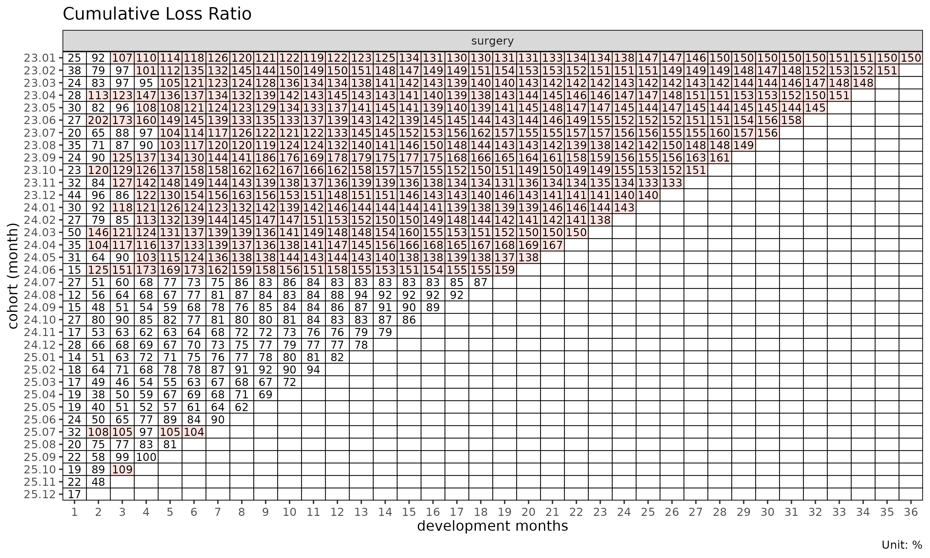
Only the upper-left region (the observed area) is filled; the empty lower-right cells are the future cells still to be projected.
Two views of loss development
To project future cells, the way “loss grows over development time” must be expressed as a model. lossratio uses two basic views.
-
Multiplicative – chain ladder (CL). The cumulative
loss at the next development period is a multiple of the current one:
C_{k+1} = f_k * C_k. Heref_kis the age-to-age factor, estimated as the ratio of cumulative loss between two adjacent development periods. -
Additive – exposure-driven (ED). The loss
increment of the next period is made proportional to premium:
Δloss = g_k * premium.g_kis the loss intensity per unit of premium.
The two are complementary. Early in development the cumulative loss is small, so the age-to-age factor swings widely; anchoring on premium makes the exposure-driven view more stable. As development matures the age-to-age factor settles, and chain ladder preserves the cohort’s own observed level well.
fit_cl() – chain ladder
fit_cl() performs a Mack (1993) chain ladder fit on the
cumulative loss.
cl <- fit_cl(tri1)
summary(cl)
#>     coverage     cohort     latest   loss_ult    reserve loss_proc_se
#>       <char>     <Date>      <num>      <num>      <num>        <num>
#>  1:  surgery 2023-01-01  410248522  410248522          0            0
#>  2:  surgery 2023-02-01  976330445 1001441303   25110858      2751819
#>  3:  surgery 2023-03-01  978486045 1026151243   47665198      3967869
#>  4:  surgery 2023-04-01 2029909919 2186771221  156861302      6942937
#>  5:  surgery 2023-05-01  624219436  697669301   73449865      4455636
#>  6:  surgery 2023-06-01  802880717  931393934  128513217     17869565
#>  7:  surgery 2023-07-01 2539141549 3050990158  511848609     35918003
#>  8:  surgery 2023-08-01  393678329  488218204   94539875     15583801
#>  9:  surgery 2023-09-01 1364052542 1751869308  387816766     38001618
#> 10:  surgery 2023-10-01  979266043 1311793843  332527800     38496097
#> 11:  surgery 2023-11-01  604685679  848103123  243417444     35719579
#> 12:  surgery 2023-12-01 1026345366 1497869029  471523663     51405333
#> 13:  surgery 2024-01-01 1912177598 2901492851  989315253     75674312
#> 14:  surgery 2024-02-01  733902485 1160045952  426143467     51719398
#> 15:  surgery 2024-03-01  415459873  686574148  271114275     41313266
#> 16:  surgery 2024-04-01 3286053526 5687484014 2401430488    122770258
#> 17:  surgery 2024-05-01 1451731153 2645801838 1194070685     93024106
#> 18:  surgery 2024-06-01  629668308 1209024555  579356247     65346187
#> 19:  surgery 2024-07-01 1250954693 2542927190 1291972497    103136528
#> 20:  surgery 2024-08-01  425346694  918120582  492773888     65317866
#> 21:  surgery 2024-09-01  278156543  635470028  357313485     56737053
#> 22:  surgery 2024-10-01  352070323  856446521  504376198     68091257
#> 23:  surgery 2024-11-01   99050501  260916096  161865595     41787166
#> 24:  surgery 2024-12-01  103194013  295637296  192443283     49617195
#> 25:  surgery 2025-01-01  227089025  710560093  483471068     83635489
#> 26:  surgery 2025-02-01  939163074 3276849152 2337686078    192418633
#> 27:  surgery 2025-03-01  112828845  434950057  322121212     72345359
#> 28:  surgery 2025-04-01   82472453  356301148  273828695     68974257
#> 29:  surgery 2025-05-01  141214851  697290587  556075736    119238986
#> 30:  surgery 2025-06-01  136406102  789468799  653062697    136628652
#> 31:  surgery 2025-07-01  149144024 1040451732  891307708    167039609
#> 32:  surgery 2025-08-01  116327076 1008356733  892029657    183653360
#> 33:  surgery 2025-09-01   67465470  783000257  715534787    179947037
#> 34:  surgery 2025-10-01  121626173 2001214863 1879588690    337103186
#> 35:  surgery 2025-11-01   15716444  449653406  433936962    194100658
#> 36:  surgery 2025-12-01    4825085  850839118  846014033    472741759
#>     coverage     cohort     latest   loss_ult    reserve loss_proc_se
#>       <char>     <Date>      <num>      <num>      <num>        <num>
#>     loss_param_se loss_total_se loss_total_cv
#>             <num>         <num>         <num>
#>  1:             0             0   0.000000000
#>  2:       4299412       5104650   0.005097304
#>  3:       5021196       6399718   0.006236623
#>  4:      11297887      13260717   0.006064062
#>  5:       3696918       5789637   0.008298541
#>  6:       8694892      19872657   0.021336469
#>  7:      30501066      47121311   0.015444596
#>  8:       5072721      16388635   0.033568259
#>  9:      20827314      43334744   0.024736288
#> 10:      16992221      42079509   0.032077837
#> 11:      11901733      37650227   0.044393454
#> 12:      22008504      55918535   0.037332059
#> 13:      43971810      87522121   0.030164514
#> 14:      18269127      54851227   0.047283667
#> 15:      11014493      42756344   0.062274911
#> 16:      92689755     153830838   0.027047256
#> 17:      45040851     103354548   0.039063601
#> 18:      20907249      68609309   0.056747655
#> 19:      45568404     112754702   0.044340515
#> 20:      16819267      67448584   0.073463753
#> 21:      11859688      57963310   0.091213288
#> 22:      16219631      69996398   0.081728860
#> 23:       5190764      42108328   0.161386470
#> 24:       6221683      50005754   0.169145620
#> 25:      15668260      85090478   0.119751276
#> 26:      75222224     206599403   0.063048188
#> 27:      10161412      73055495   0.167962950
#> 28:       8575343      69505285   0.195074548
#> 29:      19174475     120770842   0.173200161
#> 30:      22834478     138523651   0.175464377
#> 31:      31445935     169973756   0.163365345
#> 32:      32987225     186592373   0.185045993
#> 33:      27713231     182068556   0.232526816
#> 34:      80113491     346492034   0.173140846
#> 35:      21034520     195237078   0.434194593
#> 36:      66075497     477337136   0.561019265
#>     loss_param_se loss_total_se loss_total_cv
#>             <num>         <num>         <num>
summary() reports the ultimate loss per cohort with its
standard error (loss_total_se) and coefficient of variation
(loss_total_cv). The standard error follows Mack’s variance
decomposition, computed as the sum of process error and
parameter error.
The $full slot holds the cell-level result over both the
observed and projected regions.
head(cl$full[, c("cohort", "dev", "loss_obs", "loss_proj",
                 "loss_total_se", "is_observed")])
#>        cohort   dev loss_obs loss_proj loss_total_se is_observed
#>        <Date> <int>    <num>     <num>         <num>      <lgcl>
#> 1: 2023-01-01     1  1886123   1886123             0        TRUE
#> 2: 2023-01-01     2 14030514  14030514             0        TRUE
#> 3: 2023-01-01     3 24427715  24427715             0        TRUE
#> 4: 2023-01-01     4 34672477  34672477             0        TRUE
#> 5: 2023-01-01     5 44990229  44990229             0        TRUE
#> 6: 2023-01-01     6 55621697  55621697             0        TRUE
The projection curves connect each cohort’s observed values (solid) with its projection (dashed).
plot(cl)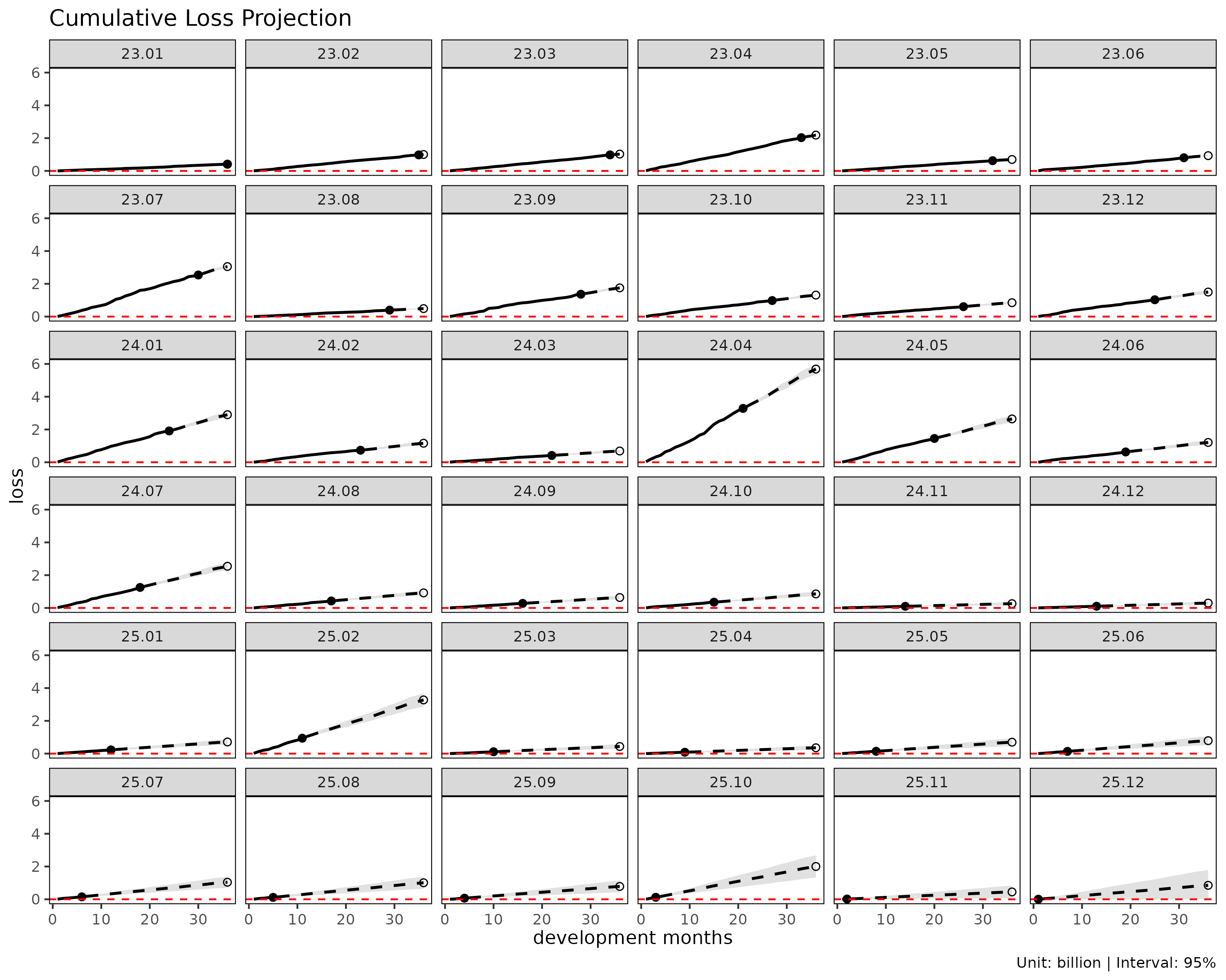
fit_ed() – exposure-driven
fit_ed() fits the same triangle with the additive
exposure-driven model.
ed <- fit_ed(tri1)
summary(ed)
#> Key: <coverage>
#>     coverage ata_from ata_to ata_link    mean  median      wt      cv       g
#>       <char>    <num>  <num>   <fctr>   <num>   <num>   <num>   <num>   <num>
#>  1:  surgery        1      2      1-2 1.34661 1.21766 1.31614 0.47327 1.31614
#>  2:  surgery        2      3      2-3 0.58109 0.56432 0.58674 0.37381 0.58674
#>  3:  surgery        3      4      3-4 0.39105 0.36751 0.38178 0.43535 0.38178
#>  4:  surgery        4      5      4-5 0.31110 0.32321 0.33127 0.35969 0.33127
#>  5:  surgery        5      6      5-6 0.27543 0.25088 0.25518 0.43531 0.25518
#>  6:  surgery        6      7      6-7 0.21364 0.20479 0.22393 0.31371 0.22393
#>  7:  surgery        7      8      7-8 0.18072 0.18227 0.19476 0.36392 0.19476
#>  8:  surgery        8      9      8-9 0.16798 0.15484 0.16849 0.67814 0.16849
#>  9:  surgery        9     10     9-10 0.14955 0.13195 0.14572 0.33906 0.14572
#> 10:  surgery       10     11    10-11 0.12550 0.12095 0.12851 0.31241 0.12851
#> 11:  surgery       11     12    11-12 0.13833 0.12898 0.14581 0.39551 0.14581
#> 12:  surgery       12     13    12-13 0.12519 0.11356 0.12075 0.34186 0.12075
#> 13:  surgery       13     14    13-14 0.11144 0.10927 0.11631 0.35239 0.11631
#> 14:  surgery       14     15    14-15 0.10561 0.09421 0.11169 0.43662 0.11169
#> 15:  surgery       15     16    15-16 0.08954 0.08726 0.08964 0.34359 0.08964
#> 16:  surgery       16     17    16-17 0.08079 0.07993 0.08162 0.24700 0.08162
#> 17:  surgery       17     18    17-18 0.08109 0.07612 0.08725 0.28780 0.08725
#> 18:  surgery       18     19    18-19 0.08636 0.08620 0.08772 0.34300 0.08772
#> 19:  surgery       19     20    19-20 0.07944 0.07838 0.08008 0.25109 0.08008
#> 20:  surgery       20     21    20-21 0.07789 0.07935 0.08007 0.32197 0.08007
#> 21:  surgery       21     22    21-22 0.06746 0.06606 0.06982 0.26290 0.06982
#> 22:  surgery       22     23    22-23 0.06748 0.06394 0.06703 0.32299 0.06703
#> 23:  surgery       23     24    23-24 0.06644 0.05971 0.06165 0.39463 0.06165
#> 24:  surgery       24     25    24-25 0.06303 0.05711 0.05902 0.45911 0.05902
#> 25:  surgery       25     26    25-26 0.06696 0.06136 0.06056 0.39347 0.06056
#> 26:  surgery       26     27    26-27 0.06265 0.05387 0.07093 0.44081 0.07093
#> 27:  surgery       27     28    27-28 0.06010 0.05136 0.06550 0.36862 0.06550
#> 28:  surgery       28     29    28-29 0.06012 0.06544 0.05404 0.31348 0.05404
#> 29:  surgery       29     30    29-30 0.05275 0.04745 0.04877 0.23587 0.04877
#> 30:  surgery       30     31    30-31 0.05437 0.04834 0.05359 0.25583 0.05359
#> 31:  surgery       31     32    31-32 0.06003 0.05618 0.05643 0.41162 0.05643
#> 32:  surgery       32     33    32-33 0.05749 0.05671 0.05622 0.07265 0.05622
#> 33:  surgery       33     34    33-34 0.04049 0.03873 0.04100 0.08481 0.04100
#> 34:  surgery       34     35    34-35 0.03562 0.03562 0.03403 0.15183 0.03403
#> 35:  surgery       35     36    35-36 0.03864 0.03864 0.03864      NA 0.03864
#>     coverage ata_from ata_to ata_link    mean  median      wt      cv       g
#>       <char>    <num>  <num>   <fctr>   <num>   <num>   <num>   <num>   <num>
#>        g_se     rse      sigma n_cohorts n_valid n_inf n_nan valid_ratio
#>       <num>   <num>      <num>     <num>   <num> <num> <num>       <num>
#>  1: 0.09107 0.06919 2930.74379        35      35     0     0           1
#>  2: 0.03508 0.05979 1580.26206        34      34     0     0           1
#>  3: 0.02931 0.07677 1587.18687        33      33     0     0           1
#>  4: 0.02135 0.06444 1319.11056        32      32     0     0           1
#>  5: 0.02087 0.08178 1421.47805        31      31     0     0           1
#>  6: 0.01273 0.05686  937.78642        30      30     0     0           1
#>  7: 0.01141 0.05860  897.25756        29      29     0     0           1
#>  8: 0.02169 0.12870 1792.82291        28      28     0     0           1
#>  9: 0.00943 0.06471  819.85457        27      27     0     0           1
#> 10: 0.00676 0.05263  614.41506        26      26     0     0           1
#> 11: 0.01185 0.08130 1065.55644        25      25     0     0           1
#> 12: 0.00987 0.08170  911.69544        24      24     0     0           1
#> 13: 0.01111 0.09556 1061.51299        23      23     0     0           1
#> 14: 0.01140 0.10209 1123.12989        22      22     0     0           1
#> 15: 0.00630 0.07031  629.63157        21      21     0     0           1
#> 16: 0.00475 0.05825  483.04483        20      20     0     0           1
#> 17: 0.00628 0.07198  644.16296        19      19     0     0           1
#> 18: 0.00745 0.08497  734.39263        18      18     0     0           1
#> 19: 0.00438 0.05473  434.93473        17      17     0     0           1
#> 20: 0.00692 0.08645  667.93909        16      16     0     0           1
#> 21: 0.00444 0.06361  392.59516        15      15     0     0           1
#> 22: 0.00501 0.07472  445.50689        14      14     0     0           1
#> 23: 0.00644 0.10443  566.66986        13      13     0     0           1
#> 24: 0.00532 0.09006  436.45244        12      12     0     0           1
#> 25: 0.00638 0.10534  505.82971        11      11     0     0           1
#> 26: 0.00878 0.12380  684.49354        10      10     0     0           1
#> 27: 0.00834 0.12727  627.18471         9       9     0     0           1
#> 28: 0.00853 0.15779  604.48158         8       8     0     0           1
#> 29: 0.00428 0.08784  300.99607         7       7     0     0           1
#> 30: 0.00553 0.10315  325.88934         6       6     0     0           1
#> 31: 0.01155 0.20459  641.18962         5       5     0     0           1
#> 32: 0.00153 0.02721   80.36415         4       4     0     0           1
#> 33: 0.00211 0.05148   81.83368         3       3     0     0           1
#> 34: 0.00348 0.10217  103.52601         2       2     0     0           1
#> 35:      NA      NA         NA         1       1     0     0           1
#>        g_se     rse      sigma n_cohorts n_valid n_inf n_nan valid_ratio
#>       <num>   <num>      <num>     <num>   <num> <num> <num>       <num>
The point projection (loss_proj) is nearly identical
between chain ladder and exposure-driven – both explain the same data.
The difference lies in how the variance accumulates. Chain
ladder amplifies variance through the square of the multiplier
f, while the exposure-driven model adds
premium-proportional increments. As a result the exposure-driven
standard error is calmer in the early development periods.
fit_sa() – stage-adaptive
fit_sa() blends the two views in a stage-adaptive (SA)
way: the development periods before the maturity point are fit with the
exposure-driven model, and the periods after it with chain ladder.
sa <- fit_sa(tri1)
summary(sa)
#>     coverage     cohort   loss_ult loss_total_se loss_total_cv
#>       <char>     <Date>      <num>         <num>         <num>
#>  1:  surgery 2023-01-01  410248522             0   0.000000000
#>  2:  surgery 2023-02-01 1001441303       5213830   0.005206903
#>  3:  surgery 2023-03-01 1026151243       6516765   0.006351412
#>  4:  surgery 2023-04-01 2186771221      13328275   0.006095671
#>  5:  surgery 2023-05-01  697669301       5934623   0.008507146
#>  6:  surgery 2023-06-01  931393934      19748953   0.021210955
#>  7:  surgery 2023-07-01 3050990158      47562095   0.015597747
#>  8:  surgery 2023-08-01  488218204      16944542   0.034721030
#>  9:  surgery 2023-09-01 1751869308      42574746   0.024314556
#> 10:  surgery 2023-10-01 1311793843      41329107   0.031518532
#> 11:  surgery 2023-11-01  848103123      37157863   0.043825274
#> 12:  surgery 2023-12-01 1497869029      57599154   0.038467355
#> 13:  surgery 2024-01-01 2901492851      88235644   0.030420598
#> 14:  surgery 2024-02-01 1160045952      54795036   0.047259587
#> 15:  surgery 2024-03-01  686574148      43001505   0.062669337
#> 16:  surgery 2024-04-01 5687484014     153573839   0.027023203
#> 17:  surgery 2024-05-01 2645801838      99819176   0.037767381
#> 18:  surgery 2024-06-01 1209024555      70198966   0.058126448
#> 19:  surgery 2024-07-01 2542927190     113847340   0.044828055
#> 20:  surgery 2024-08-01  918120582      65147845   0.071058089
#> 21:  surgery 2024-09-01  635470028      57830189   0.091140754
#> 22:  surgery 2024-10-01  856446521      72983751   0.085349352
#> 23:  surgery 2024-11-01  260916096      41722607   0.160138402
#> 24:  surgery 2024-12-01  295637296      49055982   0.166160578
#> 25:  surgery 2025-01-01  710560093      84025806   0.118458337
#> 26:  surgery 2025-02-01 3276849152     207578746   0.063455505
#> 27:  surgery 2025-03-01  434950057      72002829   0.165840618
#> 28:  surgery 2025-04-01  356301148      69341707   0.194927969
#> 29:  surgery 2025-05-01  697290587     118074803   0.169587982
#> 30:  surgery 2025-06-01  789468799     138920305   0.176211772
#> 31:  surgery 2025-07-01 1040451732     169134660   0.162761021
#> 32:  surgery 2025-08-01 1008356733     187372862   0.185979990
#> 33:  surgery 2025-09-01  783000257     182485783   0.233248980
#> 34:  surgery 2025-10-01 2001214863     340964049   0.170558023
#> 35:  surgery 2025-11-01  576954661     191871774   0.427367699
#> 36:  surgery 2025-12-01 1246569307     468598419   0.551014826
#>     coverage     cohort   loss_ult loss_total_se loss_total_cv
#>       <char>     <Date>      <num>         <num>         <num>
The maturity point is the development period where the age-to-age factor has settled sufficiently, detected automatically inside the fit (two-pass). The intuition is simple: the early region, where the age-to-age factor still swings, anchors on premium (ED); the settled region thereafter follows the cohort’s own development (CL). Stage adaptation is the package’s default workhorse for long-term loss-ratio projection.
plot(sa)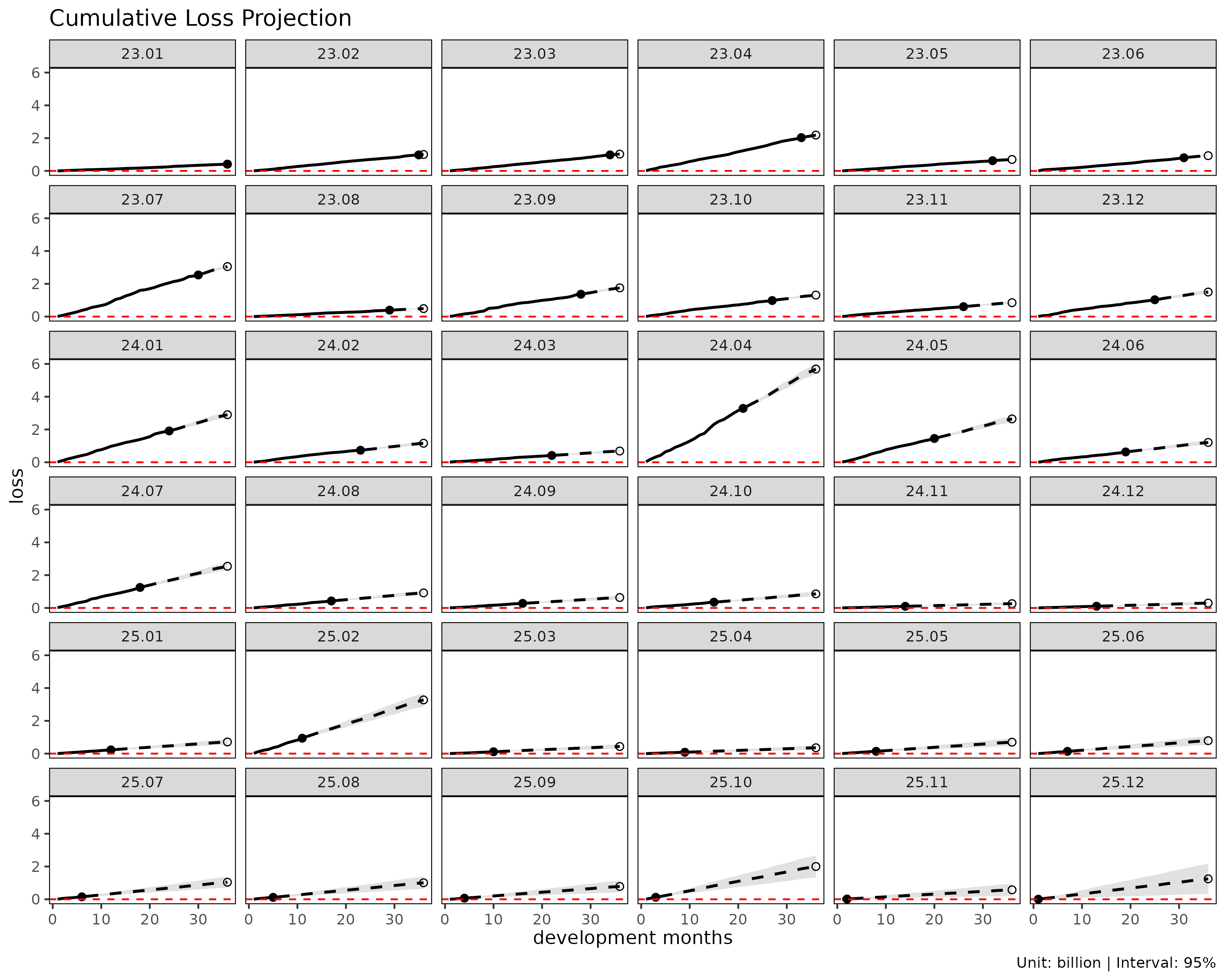
fit_bf() – Bornhuetter-Ferguson
fit_bf() brings in an external prior loss
ratio. The portion of loss that has not yet emerged is filled
not by the data but by the prior.
q_i is the emergence ratio of cohort i
(L^{obs} / L^{ult, CL}). In other words
Bornhuetter-Ferguson is a credibility blend that fills the
already-emerged part with data and the not-yet-emerged part
with the prior. The prior argument is required.
bf <- fit_bf(tri1, prior = 0.70)
summary(bf)
#>     coverage     cohort     latest   loss_ult    reserve   elr           q
#>       <char>     <Date>      <num>      <num>      <num> <num>       <num>
#>  1:  surgery 2023-01-01  410248522  410248522          0   0.7 1.000000000
#>  2:  surgery 2023-02-01  976330445  988014446   11684001   0.7 0.974925282
#>  3:  surgery 2023-03-01  978486045 1001313340   22827295   0.7 0.953549540
#>  4:  surgery 2023-04-01 2029909919 2103440848   73530929   0.7 0.928268078
#>  5:  surgery 2023-05-01  624219436  659825088   35605652   0.7 0.894721088
#>  6:  surgery 2023-06-01  802880717  860017751   57137034   0.7 0.862020556
#>  7:  surgery 2023-07-01 2539141549 2769110891  229969342   0.7 0.832235247
#>  8:  surgery 2023-08-01  393678329  438075731   44397402   0.7 0.806357333
#>  9:  surgery 2023-09-01 1364052542 1533228915  169176373   0.7 0.778626885
#> 10:  surgery 2023-10-01  979266043 1132613702  153347659   0.7 0.746509101
#> 11:  surgery 2023-11-01  604685679  731321345  126635666   0.7 0.712986030
#> 12:  surgery 2023-12-01 1026345366 1259276578  232931212   0.7 0.685203677
#> 13:  surgery 2024-01-01 1912177598 2391691252  479513654   0.7 0.659032331
#> 14:  surgery 2024-02-01  733902485  947906510  214004025   0.7 0.632649494
#> 15:  surgery 2024-03-01  415459873  541048315  125588442   0.7 0.605120181
#> 16:  surgery 2024-04-01 3286053526 4282833085  996779559   0.7 0.577769277
#> 17:  surgery 2024-05-01 1451731153 2051922702  600191549   0.7 0.548692322
#> 18:  surgery 2024-06-01  629668308  881286702  251618394   0.7 0.520806882
#> 19:  surgery 2024-07-01 1250954693 2279320912 1028366219   0.7 0.491934924
#> 20:  surgery 2024-08-01  425346694  792385329  367038635   0.7 0.463279772
#> 21:  surgery 2024-09-01  278156543  555212439  277055896   0.7 0.437717801
#> 22:  surgery 2024-10-01  352070323  758060195  405989872   0.7 0.411082670
#> 23:  surgery 2024-11-01   99050501  239786684  140736183   0.7 0.379625874
#> 24:  surgery 2024-12-01  103194013  270168423  166974410   0.7 0.349056139
#> 25:  surgery 2025-01-01  227089025  624183994  397094969   0.7 0.319591583
#> 26:  surgery 2025-02-01  939163074 2580188625 1641025551   0.7 0.286605526
#> 27:  surgery 2025-03-01  112828845  406416040  293587195   0.7 0.259406438
#> 28:  surgery 2025-04-01   82472453  338988233  256515780   0.7 0.231468390
#> 29:  surgery 2025-05-01  141214851  714552172  573337321   0.7 0.202519371
#> 30:  surgery 2025-06-01  136406102  589825915  453419813   0.7 0.172782132
#> 31:  surgery 2025-07-01  149144024  664688641  515544617   0.7 0.143345452
#> 32:  surgery 2025-08-01  116327076  758604071  642276995   0.7 0.115363018
#> 33:  surgery 2025-09-01   67465470  458478144  391012674   0.7 0.086162769
#> 34:  surgery 2025-10-01  121626173 1001607436  879981263   0.7 0.060776169
#> 35:  surgery 2025-11-01   15716444  416407427  400690983   0.7 0.034952352
#> 36:  surgery 2025-12-01    4825085  716557798  711732713   0.7 0.005670972
#>     coverage     cohort     latest   loss_ult    reserve   elr           q
#>       <char>     <Date>      <num>      <num>      <num> <num>       <num>
#>     loss_total_se loss_total_cv loss_ci_lo loss_ci_hi
#>             <num>         <num>      <num>      <num>
#>  1:             0   0.000000000  410248522  410248522
#>  2:       2706900   0.002739737  982709020  993319872
#>  3:       3577408   0.003572716  994301749 1008324932
#>  4:       6838847   0.003251267 2090036953 2116844742
#>  5:       3492508   0.005293082  652979898  666670278
#>  6:      12372795   0.014386674  835767517  884267984
#>  7:      26644265   0.009621956 2716889092 2821332690
#>  8:      10853531   0.024775468  416803200  459348261
#>  9:      26083909   0.017012404 1482105392 1584352438
#> 10:      26797039   0.023659469 1080092472 1185134933
#> 11:      26147262   0.035753452  680073652  782569037
#> 12:      36904052   0.029305756 1186945964 1331607192
#> 13:      54554640   0.022810068 2284766123 2498616381
#> 14:      37132355   0.039173014  875128432 1020684589
#> 15:      28309725   0.052323840  485562273  596534358
#> 16:      82259622   0.019206824 4121607187 4444058982
#> 17:      67184067   0.032742007 1920244351 2183601052
#> 18:      43376322   0.049219309  796270672  966302731
#> 19:      93872014   0.041184202 2095335146 2463306678
#> 20:      56754159   0.071624444  681149222  903621437
#> 21:      50204160   0.090423334  456814094  653610784
#> 22:      61451372   0.081063974  637617720  878502671
#> 23:      39077740   0.162968764  163195722  316377647
#> 24:      46347332   0.171549773  179329323  361007524
#> 25:      76064334   0.121862039  475100639  773267350
#> 26:     162339147   0.062917550 2262009743 2898367507
#> 27:      69290105   0.170490578  270609928  542222151
#> 28:      66987095   0.197608910  207695939  470280527
#> 29:     121492740   0.170026409  476430778  952673567
#> 30:     114220772   0.193651668  365957315  813694515
#> 31:     127500326   0.191819625  414792595  914584687
#> 32:     156435540   0.206215002  451996047 1065212095
#> 33:     133546948   0.291283127  196730936  720225351
#> 34:     231723393   0.231351511  547437930 1455776941
#> 35:     187300253   0.449800461   49305677  783509176
#> 36:     434845529   0.606853390 -135723778 1568839373
#>     loss_total_se loss_total_cv loss_ci_lo loss_ci_hi
#>             <num>         <num>      <num>      <num>
The prior can vary by cohort (a data frame) or be a distributional
prior (with an elr_se column). The younger a cohort – the
less data it has – the more its result is pulled toward the prior; that
is precisely the reason to use Bornhuetter-Ferguson.
fit_cc() – Cape Cod
fit_cc() has the same structure as Bornhuetter-Ferguson,
except the prior loss ratio is not supplied externally – it is
estimated by pooling the data.
cc <- fit_cc(tri1)
summary(cc)
#>     coverage     cohort     latest   loss_ult    reserve      elr           q
#>       <char>     <Date>      <num>      <num>      <num>    <num>       <num>
#>  1:  surgery 2023-01-01  410248522  410248522          0 1.355821 1.000000000
#>  2:  surgery 2023-02-01  976330445  998961036   22630591 1.355821 0.974925282
#>  3:  surgery 2023-03-01  978486045 1022699937   44213892 1.355821 0.953549540
#>  4:  surgery 2023-04-01 2029909919 2172331022  142421103 1.355821 0.928268078
#>  5:  surgery 2023-05-01  624219436  693183562   68964126 1.355821 0.894721088
#>  6:  surgery 2023-06-01  802880717  913548697  110667980 1.355821 0.862020556
#>  7:  surgery 2023-07-01 2539141549 2984566188  445424639 1.355821 0.832235247
#>  8:  surgery 2023-08-01  393678329  479671081   85992752 1.355821 0.806357333
#>  9:  surgery 2023-09-01 1364052542 1691728066  327675524 1.355821 0.778626885
#> 10:  surgery 2023-10-01  979266043 1276283138  297017095 1.355821 0.746509101
#> 11:  surgery 2023-11-01  604685679  849964659  245278980 1.355821 0.712986030
#> 12:  surgery 2023-12-01 1026345366 1477506812  451161446 1.355821 0.685203677
#> 13:  surgery 2024-01-01 1912177598 2840941382  928763784 1.355821 0.659032331
#> 14:  surgery 2024-02-01  733902485 1148404108  414501623 1.355821 0.632649494
#> 15:  surgery 2024-03-01  415459873  658710499  243250626 1.355821 0.605120181
#> 16:  surgery 2024-04-01 3286053526 5216702938 1930649412 1.355821 0.577769277
#> 17:  surgery 2024-05-01 1451731153 2614234387 1162503234 1.355821 0.548692322
#> 18:  surgery 2024-06-01  629668308 1117024715  487356407 1.355821 0.520806882
#> 19:  surgery 2024-07-01 1250954693 3242783898 1991829205 1.355821 0.491934924
#> 20:  surgery 2024-08-01  425346694 1136259071  710912377 1.355821 0.463279772
#> 21:  surgery 2024-09-01  278156543  814782518  536625975 1.355821 0.437717801
#> 22:  surgery 2024-10-01  352070323 1138426847  786356524 1.355821 0.411082670
#> 23:  surgery 2024-11-01   99050501  371640591  272590090 1.355821 0.379625874
#> 24:  surgery 2024-12-01  103194013  426604585  323410572 1.355821 0.349056139
#> 25:  surgery 2025-01-01  227089025  996217126  769128101 1.355821 0.319591583
#> 26:  surgery 2025-02-01  939163074 4117644201 3178481127 1.355821 0.286605526
#> 27:  surgery 2025-03-01  112828845  681474078  568645233 1.355821 0.259406438
#> 28:  surgery 2025-04-01   82472453  579314544  496842091 1.355821 0.231468390
#> 29:  surgery 2025-05-01  141214851 1251704480 1110489629 1.355821 0.202519371
#> 30:  surgery 2025-06-01  136406102 1014629063  878222961 1.355821 0.172782132
#> 31:  surgery 2025-07-01  149144024 1147695713  998551689 1.355821 0.143345452
#> 32:  surgery 2025-08-01  116327076 1360345066 1244017990 1.355821 0.115363018
#> 33:  surgery 2025-09-01   67465470  824812852  757347382 1.355821 0.086162769
#> 34:  surgery 2025-10-01  121626173 1826050478 1704424305 1.355821 0.060776169
#> 35:  surgery 2025-11-01   15716444  791809616  776093172 1.355821 0.034952352
#> 36:  surgery 2025-12-01    4825085 1383370954 1378545869 1.355821 0.005670972
#>     coverage     cohort     latest   loss_ult    reserve      elr           q
#>       <char>     <Date>      <num>      <num>      <num>    <num>       <num>
#>     loss_total_se loss_total_cv loss_ci_lo loss_ci_hi   elr_cc_se   elr_cc_cv
#>             <num>         <num>      <num>      <num>       <num>       <num>
#>  1:             0   0.000000000  410248522  410248522 0.004723362 0.003483765
#>  2:       4593602   0.004598379  989957742 1007964329 0.004723362 0.003483765
#>  3:       5861160   0.005731065 1011212275 1034187600 0.004723362 0.003483765
#>  4:      11606085   0.005342687 2149583513 2195078531 0.004723362 0.003483765
#>  5:       5324825   0.007681696  682747097  703620028 0.004723362 0.003483765
#>  6:      17799733   0.019484165  878661861  948435533 0.004723362 0.003483765
#>  7:      40172904   0.013460215 2905828743 3063303632 0.004723362 0.003483765
#>  8:      15331659   0.031962858  449621582  509720580 0.004723362 0.003483765
#>  9:      37557573   0.022200715 1618116576 1765339557 0.004723362 0.003483765
#> 10:      38142195   0.029885371 1201525810 1351040465 0.004723362 0.003483765
#> 11:      36892692   0.043404972  777656311  922273007 0.004723362 0.003483765
#> 12:      52372680   0.035446659 1374858246 1580155378 0.004723362 0.003483765
#> 13:      78351886   0.027579550 2687374507 2994508257 0.004723362 0.003483765
#> 14:      52317595   0.045556781 1045863507 1250944710 0.004723362 0.003483765
#> 15:      39656345   0.060202995  580985491  736435508 0.004723362 0.003483765
#> 16:     118649233   0.022744104 4984154715 5449251161 0.004723362 0.003483765
#> 17:      95166627   0.036403250 2427711225 2800757549 0.004723362 0.003483765
#> 18:      60795329   0.054426127  997868060 1236181369 0.004723362 0.003483765
#> 19:     133200048   0.041075832 2981716601 3503851194 0.004723362 0.003483765
#> 20:      79519501   0.069983601  980403712 1292114430 0.004723362 0.003483765
#> 21:      70211447   0.086172009  677170611  952394425 0.004723362 0.003483765
#> 22:      86035035   0.075573618  969801276 1307052417 0.004723362 0.003483765
#> 23:      54540884   0.146757070  264742423  478538760 0.004723362 0.003483765
#> 24:      64681286   0.151618825  299831594  553377576 0.004723362 0.003483765
#> 25:     106241396   0.106644820  787987815 1204446437 0.004723362 0.003483765
#> 26:     227653283   0.055287264 3671451966 4563836436 0.004723362 0.003483765
#> 27:      96742990   0.141961364  491861302  871086855 0.004723362 0.003483765
#> 28:      93540835   0.161468129  395977876  762651212 0.004723362 0.003483765
#> 29:     169670289   0.135551395  919156825 1584252135 0.004723362 0.003483765
#> 30:     159480991   0.157181572  702052063 1327206062 0.004723362 0.003483765
#> 31:     178077636   0.155161019  798669960 1496721466 0.004723362 0.003483765
#> 32:     218535228   0.160646908  932023889 1788666243 0.004723362 0.003483765
#> 33:     186560125   0.226184794  459161726 1190463978 0.004723362 0.003483765
#> 34:     323931990   0.177394871 1191155445 2460945512 0.004723362 0.003483765
#> 35:     261700792   0.330509742  278885490 1304733743 0.004723362 0.003483765
#> 36:     606816525   0.438650619  194032420 2572709489 0.004723362 0.003483765
#>     loss_total_se loss_total_cv loss_ci_lo loss_ci_hi   elr_cc_se   elr_cc_cv
#>             <num>         <num>      <num>      <num>       <num>       <num>
#>     elr_cc_ci_lo elr_cc_ci_hi
#>            <num>        <num>
#>  1:     1.346563     1.365079
#>  2:     1.346563     1.365079
#>  3:     1.346563     1.365079
#>  4:     1.346563     1.365079
#>  5:     1.346563     1.365079
#>  6:     1.346563     1.365079
#>  7:     1.346563     1.365079
#>  8:     1.346563     1.365079
#>  9:     1.346563     1.365079
#> 10:     1.346563     1.365079
#> 11:     1.346563     1.365079
#> 12:     1.346563     1.365079
#> 13:     1.346563     1.365079
#> 14:     1.346563     1.365079
#> 15:     1.346563     1.365079
#> 16:     1.346563     1.365079
#> 17:     1.346563     1.365079
#> 18:     1.346563     1.365079
#> 19:     1.346563     1.365079
#> 20:     1.346563     1.365079
#> 21:     1.346563     1.365079
#> 22:     1.346563     1.365079
#> 23:     1.346563     1.365079
#> 24:     1.346563     1.365079
#> 25:     1.346563     1.365079
#> 26:     1.346563     1.365079
#> 27:     1.346563     1.365079
#> 28:     1.346563     1.365079
#> 29:     1.346563     1.365079
#> 30:     1.346563     1.365079
#> 31:     1.346563     1.365079
#> 32:     1.346563     1.365079
#> 33:     1.346563     1.365079
#> 34:     1.346563     1.365079
#> 35:     1.346563     1.365079
#> 36:     1.346563     1.365079
#>     elr_cc_ci_lo elr_cc_ci_hi
#>            <num>        <num>
Apart from the absence of a prior argument, the call and
the output match Bornhuetter-Ferguson. It is the method to use when
there is no external basis for a prior and you let the portfolio speak
its own ELR.
fit_loss() / fit_premium() – the unified
dispatchers
Rather than calling a different function for each method,
fit_loss() lets you switch the method with a single
method argument.
method is one of "ed" (default),
"cl", "sa", "bf",
"cc". For "bf" / "cc" extra
arguments such as prior are forwarded through
.... fit_premium() is the companion function
that fits the premium side separately.
fe <- fit_premium(tri1)
summary(fe)
#>     coverage     cohort premium_ult premium_total_se premium_total_cv
#>       <char>     <Date>       <num>            <num>            <num>
#>  1:  surgery 2023-01-01   274192564               NA               NA
#>  2:  surgery 2023-02-01   665667720         203317.9     0.0003054339
#>  3:  surgery 2023-03-01   702047332         262601.1     0.0003740529
#>  4:  surgery 2023-04-01  1464399410        1367093.2     0.0009335767
#>  5:  surgery 2023-05-01   483147255         703451.6     0.0014560085
#>  6:  surgery 2023-06-01   591568799        1058731.8     0.0017897177
#>  7:  surgery 2023-07-01  1958263736        3910208.1     0.0019968584
#>  8:  surgery 2023-08-01   327535560        1828256.1     0.0055820892
#>  9:  surgery 2023-09-01  1091733892        3952483.5     0.0036204828
#> 10:  surgery 2023-10-01   864204933        3794976.2     0.0043913554
#> 11:  surgery 2023-11-01   630311110        3272175.4     0.0051914680
#> 12:  surgery 2023-12-01  1057060867        4484495.4     0.0042424185
#> 13:  surgery 2024-01-01  2009045340        7688434.5     0.0038268640
#> 14:  surgery 2024-02-01   832229795        4949366.6     0.0059470920
#> 15:  surgery 2024-03-01   454345985        4045484.1     0.0089042245
#> 16:  surgery 2024-04-01  3372494516       13992783.5     0.0041491213
#> 17:  surgery 2024-05-01  1899849125       10075728.1     0.0053035580
#> 18:  surgery 2024-06-01   750125230        6364391.3     0.0084844581
#> 19:  surgery 2024-07-01  2891548085       14716651.1     0.0050896560
#> 20:  surgery 2024-08-01   976935246        8364192.9     0.0085619202
#> 21:  surgery 2024-09-01   703906575        7175630.7     0.0101943622
#> 22:  surgery 2024-10-01   984833529        9313644.4     0.0094572623
#> 23:  surgery 2024-11-01   324081360        5678519.9     0.0175216881
#> 24:  surgery 2024-12-01   366444614        6236672.5     0.0170197403
#> 25:  surgery 2025-01-01   833732378       10465225.2     0.0125525791
#> 26:  surgery 2025-02-01  3286151352       23703310.8     0.0072131978
#> 27:  surgery 2025-03-01   566316398        9534760.8     0.0168363975
#> 28:  surgery 2025-04-01   476819833       10109619.3     0.0212023387
#> 29:  surgery 2025-05-01  1027051048       16264024.8     0.0158367196
#> 30:  surgery 2025-06-01   783037474       14618828.5     0.0186703135
#> 31:  surgery 2025-07-01   859730812       17196880.8     0.0200032954
#> 32:  surgery 2025-08-01  1037192185       21996644.0     0.0212094340
#> 33:  surgery 2025-09-01   611257142       18778118.6     0.0307201006
#> 34:  surgery 2025-10-01  1338462726       33336201.9     0.0249073599
#> 35:  surgery 2025-11-01   593147593       24282233.8     0.0409388868
#> 36:  surgery 2025-12-01  1022559927       47680639.5     0.0466199619
#>     coverage     cohort premium_ult premium_total_se premium_total_cv
#>       <char>     <Date>       <num>            <num>            <num>
fit_ratio() – composing the loss ratio
fit_ratio() is the composition layer: it fits the loss
side and the premium side separately, then combines them to produce the
loss ratio.
lr <- fit_ratio(tri1, method = "sa")
summary(lr)
#>     coverage     cohort     latest   loss_ult    reserve premium_ult
#>       <char>     <Date>      <num>      <num>      <num>       <num>
#>  1:  surgery 2023-01-01  410248522  410248522          0   274192564
#>  2:  surgery 2023-02-01  976330445 1001441303   25110858   665667720
#>  3:  surgery 2023-03-01  978486045 1026151243   47665198   702047332
#>  4:  surgery 2023-04-01 2029909919 2186771221  156861302  1464399410
#>  5:  surgery 2023-05-01  624219436  697669301   73449865   483147255
#>  6:  surgery 2023-06-01  802880717  931393934  128513217   591568799
#>  7:  surgery 2023-07-01 2539141549 3050990158  511848609  1958263736
#>  8:  surgery 2023-08-01  393678329  488218204   94539875   327535560
#>  9:  surgery 2023-09-01 1364052542 1751869308  387816766  1091733892
#> 10:  surgery 2023-10-01  979266043 1311793843  332527800   864204933
#> 11:  surgery 2023-11-01  604685679  848103123  243417444   630311110
#> 12:  surgery 2023-12-01 1026345366 1497869029  471523663  1057060867
#> 13:  surgery 2024-01-01 1912177598 2901492851  989315253  2009045340
#> 14:  surgery 2024-02-01  733902485 1160045952  426143467   832229795
#> 15:  surgery 2024-03-01  415459873  686574148  271114275   454345985
#> 16:  surgery 2024-04-01 3286053526 5687484014 2401430488  3372494516
#> 17:  surgery 2024-05-01 1451731153 2645801838 1194070685  1899849125
#> 18:  surgery 2024-06-01  629668308 1209024555  579356247   750125230
#> 19:  surgery 2024-07-01 1250954693 2542927190 1291972497  2891548085
#> 20:  surgery 2024-08-01  425346694  918120582  492773888   976935246
#> 21:  surgery 2024-09-01  278156543  635470028  357313485   703906575
#> 22:  surgery 2024-10-01  352070323  856446521  504376198   984833529
#> 23:  surgery 2024-11-01   99050501  260916096  161865595   324081360
#> 24:  surgery 2024-12-01  103194013  295637296  192443283   366444614
#> 25:  surgery 2025-01-01  227089025  710560093  483471068   833732378
#> 26:  surgery 2025-02-01  939163074 3276849152 2337686078  3286151352
#> 27:  surgery 2025-03-01  112828845  434950057  322121212   566316398
#> 28:  surgery 2025-04-01   82472453  356301148  273828695   476819833
#> 29:  surgery 2025-05-01  141214851  697290587  556075736  1027051048
#> 30:  surgery 2025-06-01  136406102  789468799  653062697   783037474
#> 31:  surgery 2025-07-01  149144024 1040451732  891307708   859730812
#> 32:  surgery 2025-08-01  116327076 1008356733  892029657  1037192185
#> 33:  surgery 2025-09-01   67465470  783000257  715534787   611257142
#> 34:  surgery 2025-10-01  121626173 2001214863 1879588690  1338462726
#> 35:  surgery 2025-11-01   15716444  576954661  561238217   593147593
#> 36:  surgery 2025-12-01    4825085 1246569307 1241744222  1022559927
#>     coverage     cohort     latest   loss_ult    reserve premium_ult
#>       <char>     <Date>      <num>      <num>      <num>       <num>
#>     ratio_latest ratio_ult maturity_from loss_proc_se loss_param_se
#>            <num>     <num>         <num>        <num>         <num>
#>  1:    1.4962059 1.4962059             4            0             0
#>  2:    1.5107824 1.5044162             4      2974816       4362011
#>  3:    1.4771448 1.4616554             4      4270032       5160023
#>  4:    1.5139132 1.4932888             4      7041128      11598550
#>  5:    1.4543748 1.4440097             4      4511892       3807155
#>  6:    1.5796369 1.5744474             4     17444256       9252798
#>  7:    1.5597190 1.5580078             4     35085745      32956647
#>  8:    1.4945957 1.4905808             4     15581189       5527584
#>  9:    1.6079808 1.6046670             4     37754499      22337518
#> 10:    1.5129472 1.5179199             4     36292444      18145424
#> 11:    1.3298743 1.3455310             4     36448974      12573545
#> 12:    1.3981081 1.4170130             4     50088510      23067166
#> 13:    1.4274951 1.4442147             4     77086126      45322232
#> 14:    1.3793745 1.3939010             4     52024922      19053928
#> 15:    1.4969280 1.5111263             4     41835349      11430104
#> 16:    1.6712898 1.6864324             4    128329943      96356457
#> 17:    1.3770835 1.3926379             4     88940013      45748540
#> 18:    1.5918247 1.6117636             4     64461772      21226463
#> 19:    0.8658750 0.8794345             4    102590260      46504658
#> 20:    0.9236050 0.9397968             4     64598903      17104018
#> 21:    0.8920448 0.9027761             4     55690523      12099317
#> 22:    0.8596968 0.8696358             4     66391237      16462136
#> 23:    0.7871749 0.8050944             4     41431955       5297452
#> 24:    0.7813438 0.8067721             4     49894835       6370067
#> 25:    0.8188282 0.8522640             4     85025980      15999454
#> 26:    0.9377837 0.9971693             4    182877119      76356271
#> 27:    0.7193486 0.7680337             4     69632308      10311279
#> 28:    0.6947510 0.7472448             4     70309787       8715699
#> 29:    0.6203897 0.6789250             4    118636641      19479723
#> 30:    0.8981587 1.0082133             4    132736664      23023332
#> 31:    1.0440457 1.2102064             4    165733132      31664923
#> 32:    0.8100543 0.9721985             4    185534229      32540766
#> 33:    0.9985960 1.2809670             4    184367813      27287599
#> 34:    1.0894657 1.4951592             4    330089483      80102400
#> 35:    0.4765917 0.9727000             4    197962944      20848833
#> 36:    0.1689836 1.2190672             4    476510733      64518340
#>     ratio_latest ratio_ult maturity_from loss_proc_se loss_param_se
#>            <num>     <num>         <num>        <num>         <num>
#>     loss_total_se loss_total_cv    ratio_se    ratio_cv ratio_ci_lo ratio_ci_hi
#>             <num>         <num>       <num>       <num>       <num>       <num>
#>  1:             0   0.000000000 0.000000000 0.000000000   1.4962059   1.4962059
#>  2:       5279836   0.005272237 0.007931639 0.005272237   1.4888705   1.5199619
#>  3:       6697687   0.006526998 0.009540221 0.006526998   1.4429569   1.4803538
#>  4:      13568488   0.006204804 0.009265565 0.006204804   1.4751286   1.5114490
#>  5:       5903524   0.008461780 0.012218892 0.008461780   1.4200611   1.4679582
#>  6:      19746299   0.021200803 0.033379548 0.021200803   1.5090246   1.6398701
#>  7:      48136785   0.015777430 0.024581360 0.015777430   1.5098292   1.6061864
#>  8:      16532623   0.033863185 0.050475812 0.033863185   1.3916500   1.5895115
#>  9:      43867607   0.025040456 0.040181593 0.025040456   1.5259125   1.6834214
#> 10:      40575829   0.030931560 0.046951629 0.030931560   1.4258964   1.6099434
#> 11:      38556734   0.045462318 0.061170958 0.045462318   1.2256381   1.4654238
#> 12:      55144837   0.036815526 0.052168081 0.036815526   1.3147655   1.5192606
#> 13:      89422455   0.030819464 0.044509924 0.030819464   1.3569769   1.5314526
#> 14:      55404374   0.047760500 0.066573409 0.047760500   1.2634195   1.5243825
#> 15:      43368695   0.063166805 0.095453018 0.063166805   1.3240418   1.6982107
#> 16:     160477852   0.028215965 0.047584318 0.028215965   1.5931688   1.7796959
#> 17:     100016273   0.037801876 0.052644324 0.037801876   1.2894569   1.4958188
#> 18:      67866655   0.056133397 0.090473767 0.056133397   1.4344383   1.7890889
#> 19:     112638558   0.044294842 0.038954413 0.044294842   0.8030853   0.9557838
#> 20:      66824889   0.072784436 0.068402577 0.072784436   0.8057302   1.0738634
#> 21:      56989717   0.089681204 0.080962047 0.089681204   0.7440934   1.0614588
#> 22:      68401742   0.079866916 0.069455131 0.079866916   0.7335063   1.0057654
#> 23:      41769245   0.160086887 0.128885060 0.160086887   0.5524843   1.0577045
#> 24:      50299824   0.170140320 0.137264466 0.170140320   0.5377387   1.0758055
#> 25:      86518205   0.121760574 0.103772154 0.121760574   0.6488743   1.0556537
#> 26:     198177499   0.060478066 0.060306869 0.060478066   0.8789700   1.1153686
#> 27:      70391625   0.161838408 0.124297345 0.161838408   0.5244153   1.0116520
#> 28:      70847933   0.198842842 0.148584283 0.198842842   0.4560250   1.0384647
#> 29:     120225256   0.172417723 0.117058695 0.172417723   0.4494941   0.9083558
#> 30:     134718580   0.170644590 0.172046146 0.170644590   0.6710091   1.3454176
#> 31:     168730965   0.162170872 0.196260228 0.162170872   0.8255434   1.5948694
#> 32:     188366269   0.186805188 0.181611732 0.186805188   0.6162461   1.3281510
#> 33:     186376242   0.238028328 0.304906445 0.238028328   0.6833614   1.8785727
#> 34:     339669635   0.169731717 0.253775939 0.169731717   0.9977675   1.9925509
#> 35:     199057783   0.345014602 0.335595702 0.345014602   0.3149445   1.6304555
#> 36:     480858705   0.385745664 0.470249902 0.385745664   0.2973944   2.1407401
#>     loss_total_se loss_total_cv    ratio_se    ratio_cv ratio_ci_lo ratio_ci_hi
#>             <num>         <num>       <num>       <num>       <num>       <num>
$full holds loss_proj /
premium_proj / ratio_proj together with the
loss-ratio standard error (ratio_se) and confidence
interval (ratio_ci_lo / ratio_ci_hi).
head(lr$full[, c("cohort", "dev", "loss_proj", "premium_proj",
                 "ratio_proj", "ratio_se")])
#>        cohort   dev loss_proj premium_proj ratio_proj ratio_se
#>        <Date> <int>     <num>        <num>      <num>    <num>
#> 1: 2023-01-01     1   1886123      7527562  0.2505623        0
#> 2: 2023-01-01     2  14030514     15168591  0.9249715        0
#> 3: 2023-01-01     3  24427715     22794364  1.0716559        0
#> 4: 2023-01-01     4  34672477     31558907  1.0986590        0
#> 5: 2023-01-01     5  44990229     39336754  1.1437199        0
#> 6: 2023-01-01     6  55621697     47008228  1.1832332        0
The loss-ratio standard error is governed by se_method:
"fixed" (default) treats premium as a known value, while
"delta" carries the uncertainty of premium and the
loss-premium correlation through the delta method.
plot(lr)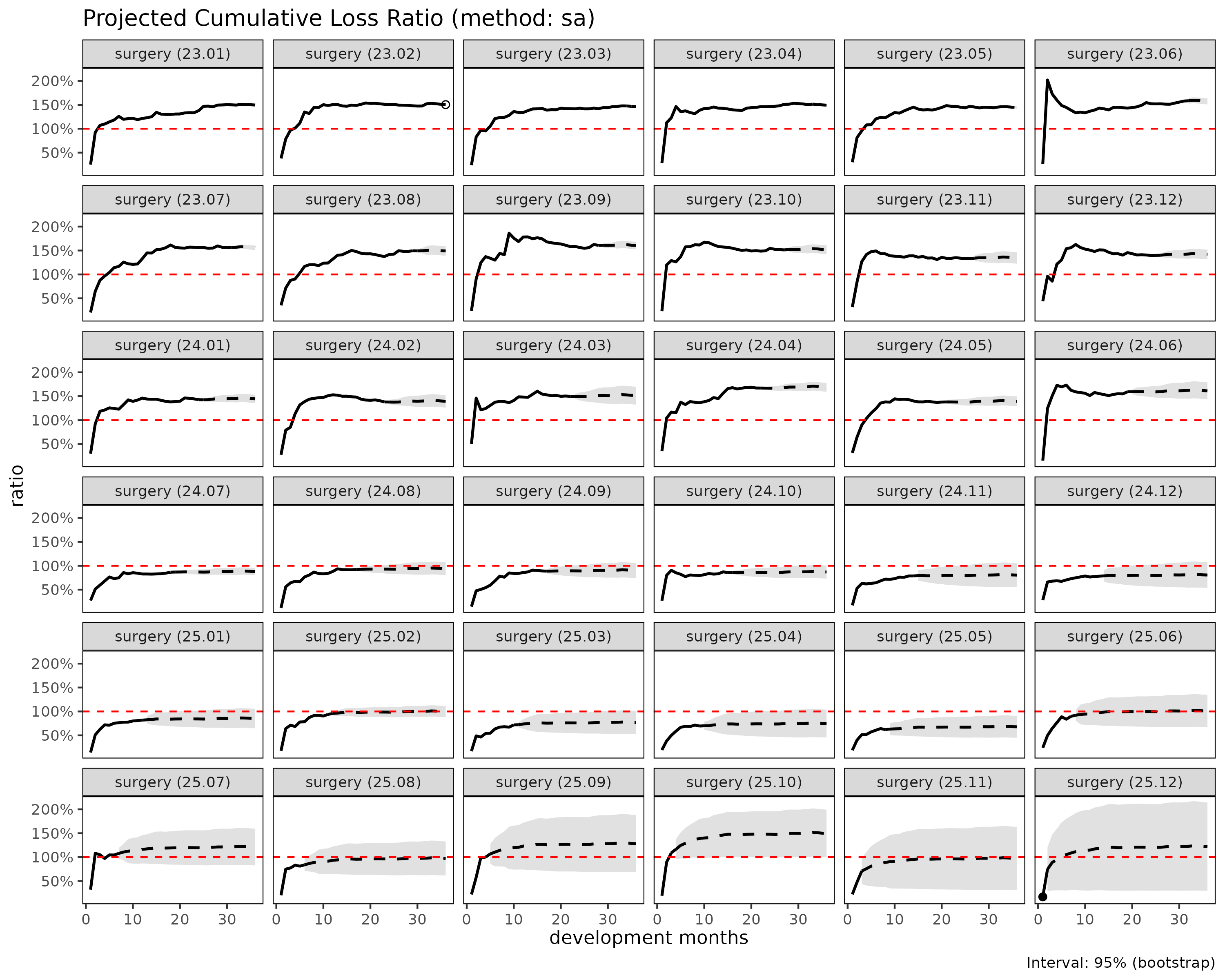
Calendar and Total – the other aggregation frameworks
The same long-format experience can be aggregated three ways
depending on the question. as_triangle() keeps both axes
(cohort x dev) for projection; two siblings collapse one or both
axes.
as_calendar() collapses cohorts onto the diagonal,
giving one row per calendar period – the diagonal sum of the triangle.
Use it for calendar-time trend and diagonal-effect analysis.
cal <- as_calendar(tri1)
head(cal)
#> shape: (6, 18)
#> ┌──────────┬────────────┬─────────┬───┬───────────────┬────────────────┐
#> │ coverage ┆ calendar   ┆ cal_idx ┆ … ┆ premium_share ┆ incr_premium_… │
#> │ <chr>    ┆ <date>     ┆ <int>   ┆ … ┆ <dbl>         ┆ <dbl>          │
#> ├──────────┼────────────┼─────────┼───┼───────────────┼────────────────┤
#> │ surgery  ┆ 2023-01-01 ┆ 1       ┆ … ┆ 1             ┆ 1              │
#> │ surgery  ┆ 2023-02-01 ┆ 2       ┆ … ┆ 1             ┆ 1              │
#> │ surgery  ┆ 2023-03-01 ┆ 3       ┆ … ┆ 1             ┆ 1              │
#> │ surgery  ┆ 2023-04-01 ┆ 4       ┆ … ┆ 1             ┆ 1              │
#> │ surgery  ┆ 2023-05-01 ┆ 5       ┆ … ┆ 1             ┆ 1              │
#> │ surgery  ┆ 2023-06-01 ┆ 6       ┆ … ┆ 1             ┆ 1              │
#> └──────────┴────────────┴─────────┴───┴───────────────┴────────────────┘
#> 13 more variables: n_cohorts <int>, loss <dbl>, incr_loss <dbl>, premium <dbl>,
#>                    incr_premium <dbl>, ratio <dbl>, incr_ratio <dbl>,
#>                    margin <dbl>, incr_margin <dbl>, profit <fct>,
#>                    incr_profit <fct>, loss_share <dbl>, incr_loss_share <dbl>
plot(cal)              # x axis: calendar (Date)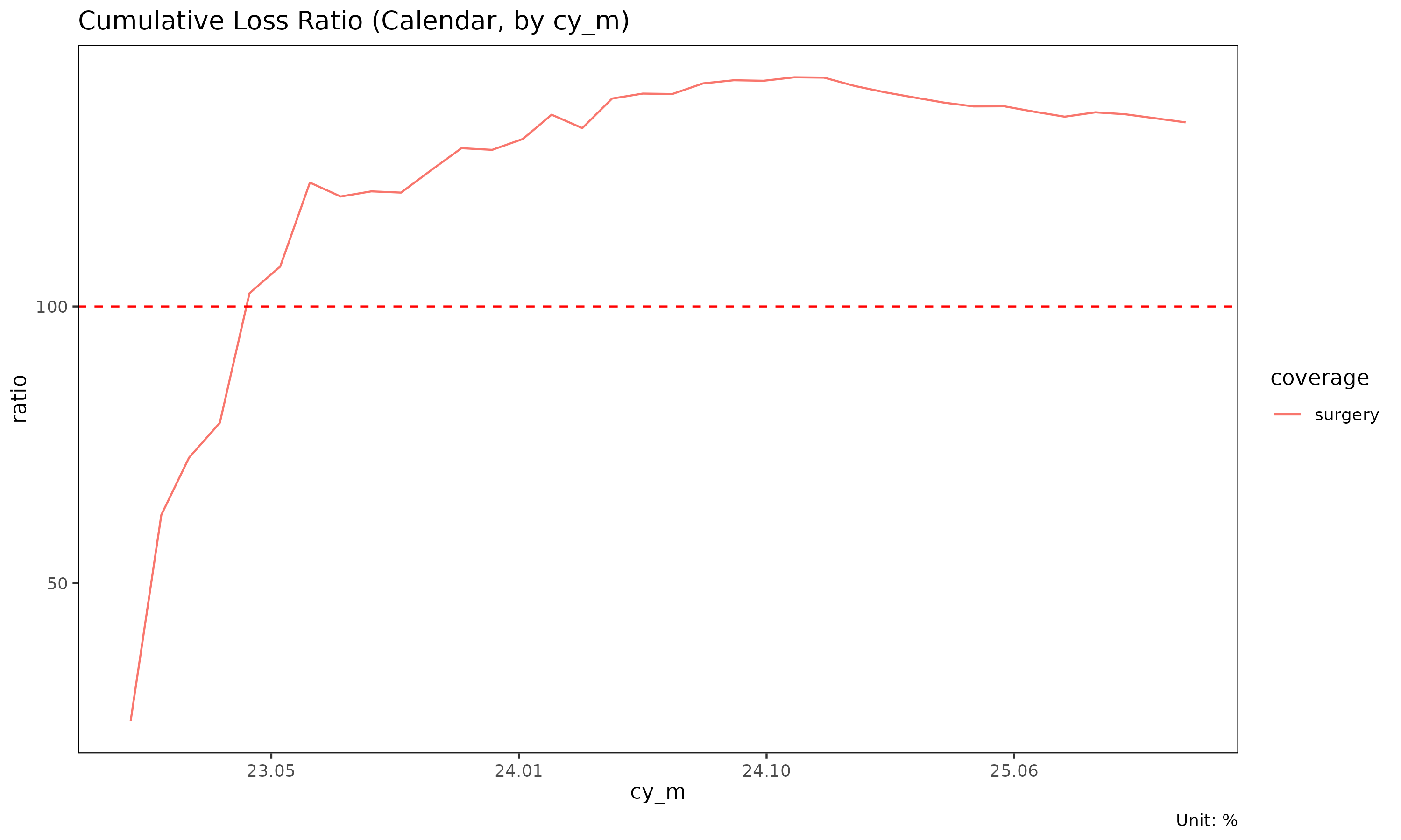
The t column is a sequential index within group (1, 2,
3, …), a time-series convention. It is not a development
period.
as_total() collapses both axes to one value per group,
useful for portfolio-level comparison. The period_from /
period_to arguments bound a fixed window so groups stay
comparable.
tot <- as_total(
  as_triangle(
    experience[uy_m >= as.Date("2023-04-01") &
               uy_m <= as.Date("2024-03-01")],
    groups = "coverage", cohort = "uy_m", dev = "dev_m",
    loss = "incr_loss", premium = "incr_premium"
  )
)
head(tot)
#> shape: (4, 9)
#> ┌───────────┬───────────┬─────────────┬───┬────────────┬───────────────┐
#> │ coverage  ┆ n_cohorts ┆ sales_start ┆ … ┆ loss_share ┆ premium_share │
#> │ <chr>     ┆ <int>     ┆ <date>      ┆ … ┆ <dbl>      ┆ <dbl>         │
#> ├───────────┼───────────┼─────────────┼───┼────────────┼───────────────┤
#> │ ci        ┆ 12        ┆ 2023-04-01  ┆ … ┆ 0.33461100 ┆ 0.427133      │
#> │ cancer    ┆ 12        ┆ 2023-04-01  ┆ … ┆ 0.11375800 ┆ 0.162389      │
#> │ inpatient ┆ 12        ┆ 2023-04-01  ┆ … ┆ 0.00644687 ┆ 0.016502      │
#> │ surgery   ┆ 12        ┆ 2023-04-01  ┆ … ┆ 0.54518400 ┆ 0.393976      │
#> └───────────┴───────────┴─────────────┴───┴────────────┴───────────────┘
#> 4 more variables: sales_end <date>, loss <dbl>, premium <dbl>, ratio <dbl>
The Link object – factor-level diagnostics
Between a Triangle and a fit sits the Link object,
the per-link factor table built by as_link(). It is the
intermediate object that feeds both chain ladder and the exposure-driven
model.
# single-variable mode -> observed age-to-age factors
ata <- as_link(tri1, loss = "loss")
summary(ata, model = "ata")
#> Key: <coverage>
#>     coverage ata_from ata_to ata_link  mean median    wt    cv     f  f_se
#>       <char>    <num>  <num>   <fctr> <num>  <num> <num> <num> <num> <num>
#>  1:  surgery        1      2      1-2 6.595  6.089 6.163 0.427 6.163 0.382
#>  2:  surgery        2      3      2-3 1.765  1.768 1.739 0.157 1.739 0.042
#>  3:  surgery        3      4      3-4 1.435  1.400 1.418 0.105 1.418 0.027
#>  4:  surgery        4      5      4-5 1.324  1.331 1.339 0.068 1.339 0.018
#>  5:  surgery        5      6      5-6 1.267  1.246 1.243 0.070 1.243 0.016
#>  6:  surgery        6      7      6-7 1.204  1.194 1.205 0.048 1.205 0.011
#>  7:  surgery        7      8      7-8 1.163  1.158 1.172 0.045 1.172 0.011
#>  8:  surgery        8      9      8-9 1.141  1.124 1.143 0.066 1.143 0.015
#>  9:  surgery        9     10     9-10 1.127  1.131 1.121 0.030 1.121 0.006
#> 10:  surgery       10     11    10-11 1.104  1.098 1.105 0.025 1.105 0.005
#> 11:  surgery       11     12    11-12 1.110  1.108 1.115 0.029 1.115 0.007
#> 12:  surgery       12     13    12-13 1.099  1.094 1.092 0.028 1.092 0.007
#> 13:  surgery       13     14    13-14 1.085  1.078 1.088 0.026 1.088 0.007
#> 14:  surgery       14     15    14-15 1.077  1.070 1.083 0.026 1.083 0.007
#> 15:  surgery       15     16    15-16 1.064  1.063 1.065 0.018 1.065 0.003
#> 16:  surgery       16     17    16-17 1.058  1.057 1.058 0.015 1.058 0.004
#> 17:  surgery       17     18    17-18 1.057  1.055 1.062 0.015 1.062 0.004
#> 18:  surgery       18     19    18-19 1.059  1.060 1.059 0.019 1.059 0.005
#> 19:  surgery       19     20    19-20 1.055  1.057 1.054 0.015 1.054 0.003
#> 20:  surgery       20     21    20-21 1.053  1.053 1.053 0.018 1.053 0.005
#> 21:  surgery       21     22    21-22 1.046  1.046 1.047 0.012 1.047 0.003
#> 22:  surgery       22     23    22-23 1.046  1.044 1.045 0.013 1.045 0.003
#> 23:  surgery       23     24    23-24 1.046  1.040 1.042 0.018 1.042 0.004
#> 24:  surgery       24     25    24-25 1.043  1.040 1.040 0.021 1.040 0.004
#> 25:  surgery       25     26    25-26 1.046  1.042 1.041 0.018 1.041 0.005
#> 26:  surgery       26     27    26-27 1.042  1.036 1.047 0.017 1.047 0.006
#> 27:  surgery       27     28    27-28 1.040  1.034 1.043 0.014 1.043 0.005
#> 28:  surgery       28     29    28-29 1.041  1.045 1.036 0.013 1.036 0.006
#> 29:  surgery       29     30    29-30 1.035  1.033 1.032 0.008 1.032 0.003
#> 30:  surgery       30     31    30-31 1.036  1.032 1.036 0.009 1.036 0.004
#> 31:  surgery       31     32    31-32 1.041  1.038 1.038 0.016 1.038 0.008
#> 32:  surgery       32     33    32-33 1.038  1.038 1.037 0.003 1.037 0.001
#> 33:  surgery       33     34    33-34 1.027  1.026 1.027 0.003 1.027 0.002
#> 34:  surgery       34     35    34-35 1.024  1.024 1.022 0.004 1.022 0.002
#> 35:  surgery       35     36    35-36 1.026  1.026 1.026    NA 1.026    NA
#>     coverage ata_from ata_to ata_link  mean median    wt    cv     f  f_se
#>       <char>    <num>  <num>   <fctr> <num>  <num> <num> <num> <num> <num>
#>       rse    sigma n_cohorts n_valid n_inf n_nan valid_ratio
#>     <num>    <num>     <num>   <num> <num> <num>       <num>
#>  1: 0.062 6207.618        35      35     0     0           1
#>  2: 0.024 1689.250        34      34     0     0           1
#>  3: 0.019 1372.883        33      33     0     0           1
#>  4: 0.014 1105.053        32      32     0     0           1
#>  5: 0.013 1086.826        31      31     0     0           1
#>  6: 0.009  812.770        30      30     0     0           1
#>  7: 0.009  879.041        29      29     0     0           1
#>  8: 0.013 1364.524        28      28     0     0           1
#>  9: 0.006  619.261        27      27     0     0           1
#> 10: 0.004  482.198        26      26     0     0           1
#> 11: 0.006  720.023        25      25     0     0           1
#> 12: 0.007  760.455        24      24     0     0           1
#> 13: 0.007  821.580        23      23     0     0           1
#> 14: 0.006  754.516        22      22     0     0           1
#> 15: 0.003  402.657        21      21     0     0           1
#> 16: 0.004  453.146        20      20     0     0           1
#> 17: 0.004  492.253        19      19     0     0           1
#> 18: 0.005  599.191        18      18     0     0           1
#> 19: 0.003  388.598        17      17     0     0           1
#> 20: 0.005  614.425        16      16     0     0           1
#> 21: 0.003  322.569        15      15     0     0           1
#> 22: 0.003  345.135        14      14     0     0           1
#> 23: 0.004  477.542        13      13     0     0           1
#> 24: 0.004  386.326        12      12     0     0           1
#> 25: 0.004  439.006        11      11     0     0           1
#> 26: 0.005  541.166        10      10     0     0           1
#> 27: 0.005  498.003         9       9     0     0           1
#> 28: 0.006  522.482         8       8     0     0           1
#> 29: 0.003  253.107         7       7     0     0           1
#> 30: 0.004  267.272         6       6     0     0           1
#> 31: 0.008  540.332         5       5     0     0           1
#> 32: 0.001   78.583         4       4     0     0           1
#> 33: 0.002   81.016         3       3     0     0           1
#> 34: 0.002   88.069         2       2     0     0           1
#> 35:    NA       NA         1       1     0     0           1
#>       rse    sigma n_cohorts n_valid n_inf n_nan valid_ratio
#>     <num>    <num>     <num>   <num> <num> <num>       <num>

# dual-variable mode -> exposure-driven intensities g_k
ed_link <- as_link(tri1, loss = "loss", exposure = "premium")
summary(ed_link, model = "ed")
#> Key: <coverage>
#>     coverage ata_from ata_to ata_link    mean  median      wt      cv       g
#>       <char>    <num>  <num>   <fctr>   <num>   <num>   <num>   <num>   <num>
#>  1:  surgery        1      2      1-2 1.34661 1.21766 1.31614 0.47327 1.31614
#>  2:  surgery        2      3      2-3 0.58109 0.56432 0.58674 0.37381 0.58674
#>  3:  surgery        3      4      3-4 0.39105 0.36751 0.38178 0.43535 0.38178
#>  4:  surgery        4      5      4-5 0.31110 0.32321 0.33127 0.35969 0.33127
#>  5:  surgery        5      6      5-6 0.27543 0.25088 0.25518 0.43531 0.25518
#>  6:  surgery        6      7      6-7 0.21364 0.20479 0.22393 0.31371 0.22393
#>  7:  surgery        7      8      7-8 0.18072 0.18227 0.19476 0.36392 0.19476
#>  8:  surgery        8      9      8-9 0.16798 0.15484 0.16849 0.67814 0.16849
#>  9:  surgery        9     10     9-10 0.14955 0.13195 0.14572 0.33906 0.14572
#> 10:  surgery       10     11    10-11 0.12550 0.12095 0.12851 0.31241 0.12851
#> 11:  surgery       11     12    11-12 0.13833 0.12898 0.14581 0.39551 0.14581
#> 12:  surgery       12     13    12-13 0.12519 0.11356 0.12075 0.34186 0.12075
#> 13:  surgery       13     14    13-14 0.11144 0.10927 0.11631 0.35239 0.11631
#> 14:  surgery       14     15    14-15 0.10561 0.09421 0.11169 0.43662 0.11169
#> 15:  surgery       15     16    15-16 0.08954 0.08726 0.08964 0.34359 0.08964
#> 16:  surgery       16     17    16-17 0.08079 0.07993 0.08162 0.24700 0.08162
#> 17:  surgery       17     18    17-18 0.08109 0.07612 0.08725 0.28780 0.08725
#> 18:  surgery       18     19    18-19 0.08636 0.08620 0.08772 0.34300 0.08772
#> 19:  surgery       19     20    19-20 0.07944 0.07838 0.08008 0.25109 0.08008
#> 20:  surgery       20     21    20-21 0.07789 0.07935 0.08007 0.32197 0.08007
#> 21:  surgery       21     22    21-22 0.06746 0.06606 0.06982 0.26290 0.06982
#> 22:  surgery       22     23    22-23 0.06748 0.06394 0.06703 0.32299 0.06703
#> 23:  surgery       23     24    23-24 0.06644 0.05971 0.06165 0.39463 0.06165
#> 24:  surgery       24     25    24-25 0.06303 0.05711 0.05902 0.45911 0.05902
#> 25:  surgery       25     26    25-26 0.06696 0.06136 0.06056 0.39347 0.06056
#> 26:  surgery       26     27    26-27 0.06265 0.05387 0.07093 0.44081 0.07093
#> 27:  surgery       27     28    27-28 0.06010 0.05136 0.06550 0.36862 0.06550
#> 28:  surgery       28     29    28-29 0.06012 0.06544 0.05404 0.31348 0.05404
#> 29:  surgery       29     30    29-30 0.05275 0.04745 0.04877 0.23587 0.04877
#> 30:  surgery       30     31    30-31 0.05437 0.04834 0.05359 0.25583 0.05359
#> 31:  surgery       31     32    31-32 0.06003 0.05618 0.05643 0.41162 0.05643
#> 32:  surgery       32     33    32-33 0.05749 0.05671 0.05622 0.07265 0.05622
#> 33:  surgery       33     34    33-34 0.04049 0.03873 0.04100 0.08481 0.04100
#> 34:  surgery       34     35    34-35 0.03562 0.03562 0.03403 0.15183 0.03403
#> 35:  surgery       35     36    35-36 0.03864 0.03864 0.03864      NA 0.03864
#>     coverage ata_from ata_to ata_link    mean  median      wt      cv       g
#>       <char>    <num>  <num>   <fctr>   <num>   <num>   <num>   <num>   <num>
#>        g_se     rse      sigma n_cohorts n_valid n_inf n_nan valid_ratio
#>       <num>   <num>      <num>     <num>   <num> <num> <num>       <num>
#>  1: 0.09107 0.06919 2930.74379        35      35     0     0           1
#>  2: 0.03508 0.05979 1580.26206        34      34     0     0           1
#>  3: 0.02931 0.07677 1587.18687        33      33     0     0           1
#>  4: 0.02135 0.06444 1319.11056        32      32     0     0           1
#>  5: 0.02087 0.08178 1421.47805        31      31     0     0           1
#>  6: 0.01273 0.05686  937.78642        30      30     0     0           1
#>  7: 0.01141 0.05860  897.25756        29      29     0     0           1
#>  8: 0.02169 0.12870 1792.82291        28      28     0     0           1
#>  9: 0.00943 0.06471  819.85457        27      27     0     0           1
#> 10: 0.00676 0.05263  614.41506        26      26     0     0           1
#> 11: 0.01185 0.08130 1065.55644        25      25     0     0           1
#> 12: 0.00987 0.08170  911.69544        24      24     0     0           1
#> 13: 0.01111 0.09556 1061.51299        23      23     0     0           1
#> 14: 0.01140 0.10209 1123.12989        22      22     0     0           1
#> 15: 0.00630 0.07031  629.63157        21      21     0     0           1
#> 16: 0.00475 0.05825  483.04483        20      20     0     0           1
#> 17: 0.00628 0.07198  644.16296        19      19     0     0           1
#> 18: 0.00745 0.08497  734.39263        18      18     0     0           1
#> 19: 0.00438 0.05473  434.93473        17      17     0     0           1
#> 20: 0.00692 0.08645  667.93909        16      16     0     0           1
#> 21: 0.00444 0.06361  392.59516        15      15     0     0           1
#> 22: 0.00501 0.07472  445.50689        14      14     0     0           1
#> 23: 0.00644 0.10443  566.66986        13      13     0     0           1
#> 24: 0.00532 0.09006  436.45244        12      12     0     0           1
#> 25: 0.00638 0.10534  505.82971        11      11     0     0           1
#> 26: 0.00878 0.12380  684.49354        10      10     0     0           1
#> 27: 0.00834 0.12727  627.18471         9       9     0     0           1
#> 28: 0.00853 0.15779  604.48158         8       8     0     0           1
#> 29: 0.00428 0.08784  300.99607         7       7     0     0           1
#> 30: 0.00553 0.10315  325.88934         6       6     0     0           1
#> 31: 0.01155 0.20459  641.18962         5       5     0     0           1
#> 32: 0.00153 0.02721   80.36415         4       4     0     0           1
#> 33: 0.00211 0.05148   81.83368         3       3     0     0           1
#> 34: 0.00348 0.10217  103.52601         2       2     0     0           1
#> 35:      NA      NA         NA         1       1     0     0           1
#>        g_se     rse      sigma n_cohorts n_valid n_inf n_nan valid_ratio
#>       <num>   <num>      <num>     <num>   <num> <num> <num>       <num>
In single-variable mode (loss only) the Link carries the
observed age-to-age factors. Supplying exposure adds the
exposure-driven intensity
intensity = loss_delta / premium_from. The
summary() method computes the per-link statistics – mean /
median / weighted factor, coefficient of variation, WLS standard error –
that drive maturity detection. The factor-level helpers
fit_ata() and fit_intensity() wrap this same
machinery and return per-link estimates only (no $full
projection).
Diagnostics – maturity, convergence, regime
There are diagnostic functions for inspecting the triangle’s structure before and after fitting.
Maturity point – the development period where the age-to-age factor settles. It is also the stage-switch point of the stage-adaptive method.
detect_maturity(tri1)
#> Key: <coverage>
#>    coverage ata_from change ata_link     mean   median       wt        cv
#>      <char>    <num>  <num>   <char>    <num>    <num>    <num>     <num>
#> 1:  surgery        3      4      3-4 1.434507 1.400098 1.417706 0.1053282
#>           f       f_se        rse    sigma n_cohorts n_valid n_inf n_nan
#>       <num>      <num>      <num>    <num>     <num>   <num> <num> <num>
#> 1: 1.417706 0.02651852 0.01870522 1372.883        33      33     0     0
#>    valid_ratio
#>          <num>
#> 1:           1
Convergence point – the development period beyond which the projected loss ratio no longer moves meaningfully. As the denominator of the cumulative loss ratio grows it dampens the signal – an inertia effect – which a dual criterion is used to filter through.
detect_convergence(tri1)
#> <Convergence>
#>   method     : tail
#>   conv_k     : NA
#>   mat_k      : 4
#>   dev_max    : 36
#>   candidates : 31
#>   passes :
#>     window :  0/31 (drift_window < 0.01  & dispersion < 0.15)
#>     tail   :  0/31 (drift_tail   < 0.01  & dispersion < 0.15)  <- method
#>     slope  :  1/31 (|slope|      < 0.001 & dispersion < 0.15)
#>     all    :  0/31 (window AND tail AND slope)
Regime – a structural change between underwriting cohorts. It detects whether a premium, policy-wording, or underwriting-guideline change altered the loss behaviour of cohorts after a certain point.
reg <- detect_regime(tri)
reg$changes
#>    coverage     change regime_id pre_value post_value magnitude
#>      <char>     <Date>     <int>     <num>      <num>     <num>
#> 1:  surgery 2024-07-01         2 0.9065895  0.5479919 0.3585976
The surgery product in experience has a synthetic regime
change planted during 2024, so the result above picks up that change
point.
backtest() – validation
backtest() hides the latest few calendar diagonals,
refits the model, and compares the withheld actuals against the
projection to measure the model’s accuracy.
bt <- backtest(tri1, holdout = 6L, target = "ratio", loss_method = "sa")
summary(bt)
#> Backtest summary
#>   dispatcher: fit_ratio
#>   target    : ratio
#>   holdout   : 6 diagonals (159 cells)
#>
#> By dev:
#>     coverage   dev     n      aeg_mean       aeg_med   ae_err_mean
#>       <char> <int> <int>         <num>         <num>         <num>
#>  1:  surgery     2     1 -0.2879720892 -0.2879720892 -0.3667493406
#>  2:  surgery     3     2 -0.1058236209 -0.1058236209 -0.0901195589
#>  3:  surgery     4     3 -0.0438970022  0.0217666029 -0.0230071083
#>  4:  surgery     5     4 -0.0110558266  0.0054351372  0.0118645748
#>  5:  surgery     6     5 -0.0160114000  0.0370902061  0.0134987613
#>  6:  surgery     7     6  0.0066390570  0.0520519271  0.0354091701
#>  7:  surgery     8     6  0.0387556832  0.0468493428  0.0591624141
#>  8:  surgery     9     6  0.0165983758  0.0181339640  0.0244533252
#>  9:  surgery    10     6  0.0177699119  0.0134168699  0.0253607766
#> 10:  surgery    11     6  0.0191431289  0.0114886577  0.0231290386
#> 11:  surgery    12     6  0.0007211923  0.0015017408  0.0006387361
#> 12:  surgery    13     6  0.0157220903  0.0076137593  0.0186533032
#> 13:  surgery    14     6  0.0146558512  0.0269373691  0.0203566313
#> 14:  surgery    15     6 -0.0164147403 -0.0078793254 -0.0085724729
#> 15:  surgery    16     6 -0.0053773998 -0.0036509669 -0.0020439585
#> 16:  surgery    17     6  0.0030866922 -0.0028402355  0.0055714790
#> 17:  surgery    18     6 -0.0125129664 -0.0247929775 -0.0069398934
#> 18:  surgery    19     6 -0.0113103120 -0.0086054969 -0.0082932779
#> 19:  surgery    20     6 -0.0211209295 -0.0300370470 -0.0146794960
#> 20:  surgery    21     6 -0.0123320969 -0.0288302132 -0.0081315596
#> 21:  surgery    22     6 -0.0265367863 -0.0357010146 -0.0174246731
#> 22:  surgery    23     6 -0.0241615696 -0.0113727688 -0.0160124793
#> 23:  surgery    24     6  0.0023608518  0.0086349370  0.0019991795
#> 24:  surgery    25     6 -0.0122696331 -0.0177060339 -0.0080061801
#> 25:  surgery    26     6  0.0028673644 -0.0154389229  0.0029017289
#> 26:  surgery    27     6 -0.0022551943 -0.0219579321 -0.0005984627
#> 27:  surgery    28     6  0.0021536077  0.0005528274  0.0021335463
#> 28:  surgery    29     6  0.0179714842  0.0123131943  0.0130930298
#> 29:  surgery    30     6 -0.0039272898  0.0020727095 -0.0024107193
#>     coverage   dev     n      aeg_mean       aeg_med   ae_err_mean
#>       <char> <int> <int>         <num>         <num>         <num>
#>        ae_err_med     ae_err_wt incr_aeg_mean incr_aeg_med incr_ae_err_mean
#>             <num>         <num>         <num>        <num>            <num>
#>  1: -0.3667493406 -0.3667493406   -0.57495418 -0.574954175      -0.42911219
#>  2: -0.0901195589 -0.1544635152   -0.03295105 -0.032951048       0.03104206
#>  3:  0.0437848471 -0.0656622116    0.03896663 -0.060404427       0.07170889
#>  4:  0.0123517418 -0.0162647786    0.07049188  0.081146126       0.09271533
#>  5:  0.0621128725 -0.0220352052   -0.04049602  0.091444980       0.04486252
#>  6:  0.0757446843  0.0088632803    0.12761981  0.080299453       0.16250805
#>  7:  0.0725907702  0.0550856653    0.02069969  0.007197477       0.01564729
#>  8:  0.0277518849  0.0223891429   -0.10613396 -0.136121764      -0.13147267
#>  9:  0.0171529396  0.0229537555    0.11236174  0.105535088       0.15605437
#> 10:  0.0154512077  0.0237389543    0.15969892  0.189675674       0.19686096
#> 11:  0.0018922252  0.0008808334   -0.08257465 -0.094057006      -0.08660181
#> 12:  0.0090087054  0.0190934981    0.17134975  0.064672398       0.19168084
#> 13:  0.0321857613  0.0152643056   -0.02644494 -0.114754500       0.01007152
#> 14: -0.0079107504 -0.0151493835   -0.41106393 -0.321970213      -0.28852360
#> 15: -0.0044851592 -0.0044371719    0.19818694  0.117799240       0.15063258
#> 16: -0.0018539369  0.0023518033    0.15672998  0.256737634       0.16971640
#> 17: -0.0169311833 -0.0088467233   -0.13589998 -0.185237736      -0.06313735
#> 18: -0.0054623225 -0.0075105462    0.06448340  0.048368896       0.03305654
#> 19: -0.0209835277 -0.0141893838   -0.17389925 -0.113722964      -0.11085823
#> 20: -0.0195936468 -0.0083339178    0.04888552 -0.116631342       0.04109121
#> 21: -0.0241489266 -0.0181905096   -0.22822576 -0.207832035      -0.14657964
#> 22: -0.0079804501 -0.0164674504   -0.14845744 -0.096634453      -0.09654333
#> 23:  0.0070443849  0.0016326821    0.16627897 -0.261922846       0.12001108
#> 24: -0.0128789134 -0.0083069614   -0.21608907 -0.189756124      -0.13659900
#> 25: -0.0098650416  0.0019209162    0.07312011 -0.164382561       0.05824859
#> 26: -0.0142767203 -0.0014781843   -0.32083035 -0.625762580      -0.17477888
#> 27:  0.0004018279  0.0014147005    0.06914757 -0.017229197       0.04186226
#> 28:  0.0081992616  0.0120992517    0.44252486  0.663837977       0.34283700
#> 29:  0.0012135586 -0.0026098433   -0.14700411 -0.270271875      -0.09019624
#>        ae_err_med     ae_err_wt incr_aeg_mean incr_aeg_med incr_ae_err_mean
#>             <num>         <num>         <num>        <num>            <num>
#>     incr_ae_err_med incr_ae_err_wt
#>               <num>          <num>
#>  1:    -0.429112189    -0.42911219
#>  2:     0.031042058    -0.03788330
#>  3:    -0.051312889     0.04819216
#>  4:     0.101566115     0.08262484
#>  5:     0.130130156    -0.04711615
#>  6:     0.136743653     0.14894131
#>  7:     0.008088929     0.02505782
#>  8:    -0.163940480    -0.12387084
#>  9:     0.125264952     0.13525827
#> 10:     0.236016698     0.19825482
#> 11:    -0.093881374    -0.08139958
#> 12:     0.070449982     0.19355031
#> 13:    -0.124397482    -0.02436243
#> 14:    -0.299928631    -0.30564120
#> 15:     0.148772947     0.17845143
#> 16:     0.285614433     0.13524568
#> 17:    -0.124958477    -0.09463269
#> 18:     0.033222595     0.04168906
#> 19:    -0.074261725    -0.11230739
#> 20:    -0.069418132     0.03288272
#> 21:    -0.133308413    -0.14878192
#> 22:    -0.064872712    -0.09810761
#> 23:    -0.190149810     0.11735901
#> 24:    -0.131504726    -0.14062139
#> 25:    -0.103229976     0.04391763
#> 26:    -0.317754317    -0.16402220
#> 27:    -0.009548040     0.04577902
#> 28:     0.509453512     0.33144073
#> 29:    -0.165797630    -0.08977373
#>     incr_ae_err_med incr_ae_err_wt
#>               <num>          <num>
#>
#> By calendar diagonal:
#>    coverage cal_idx     n      aeg_mean       aeg_med  ae_err_mean   ae_err_med
#>      <char>   <int> <int>         <num>         <num>        <num>        <num>
#> 1:  surgery      31    29 -0.0125686252 -0.0056732350 -0.011309410 -0.003699313
#> 2:  surgery      32    28 -0.0104717812 -0.0114871218 -0.002794292 -0.009588959
#> 3:  surgery      33    27  0.0004718616  0.0050471735  0.007666312  0.006154835
#> 4:  surgery      34    26  0.0012851467 -0.0002953897  0.008094503  0.000421251
#> 5:  surgery      35    25 -0.0006986581  0.0145835308  0.007408947  0.009455704
#> 6:  surgery      36    24 -0.0027175011  0.0105940082  0.005874139  0.009450279
#>        ae_err_wt incr_aeg_mean incr_aeg_med incr_ae_err_mean incr_ae_err_med
#>            <num>         <num>        <num>            <num>           <num>
#> 1: -0.0107004533   -0.08350070  -0.07460811     -0.036347452     -0.06750071
#> 2: -0.0089044278   -0.07573837  -0.07440057     -0.003857981     -0.07262916
#> 3:  0.0004012161    0.18105966   0.09849605      0.147072061      0.12954698
#> 4:  0.0010973317    0.01407124  -0.02312661      0.017058138     -0.02473897
#> 5: -0.0005997009   -0.03104560  -0.09210258     -0.008476082     -0.07819464
#> 6: -0.0023535415   -0.06224227  -0.09299902     -0.016968983     -0.09358995
#>    incr_ae_err_wt
#>             <num>
#> 1:    -0.06558617
#> 2:    -0.06014060
#> 3:     0.14477037
#> 4:     0.01130928
#> 5:    -0.02508022
#> 6:    -0.05088339
target is one of "ratio" /
"loss" / "premium", calling
fit_ratio / fit_loss /
fit_premium internally. The resulting A/E error tables show
which development periods and which diagonals the model missed.
plot(bt)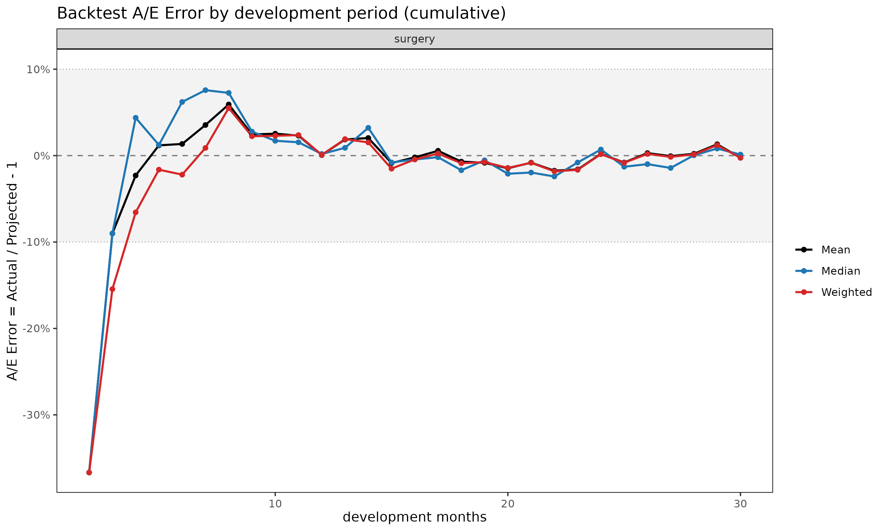
Visualisation – plot() /
plot_triangle()
Every major object supports two families of plots.
-
plot(x)– trajectory / diagnostic charts (per-cohort development curves, regime PCA, and so on). -
plot_triangle(x)– triangular heatmaps (cell values or cell status).
plot_triangle(sa, label_style = "cv")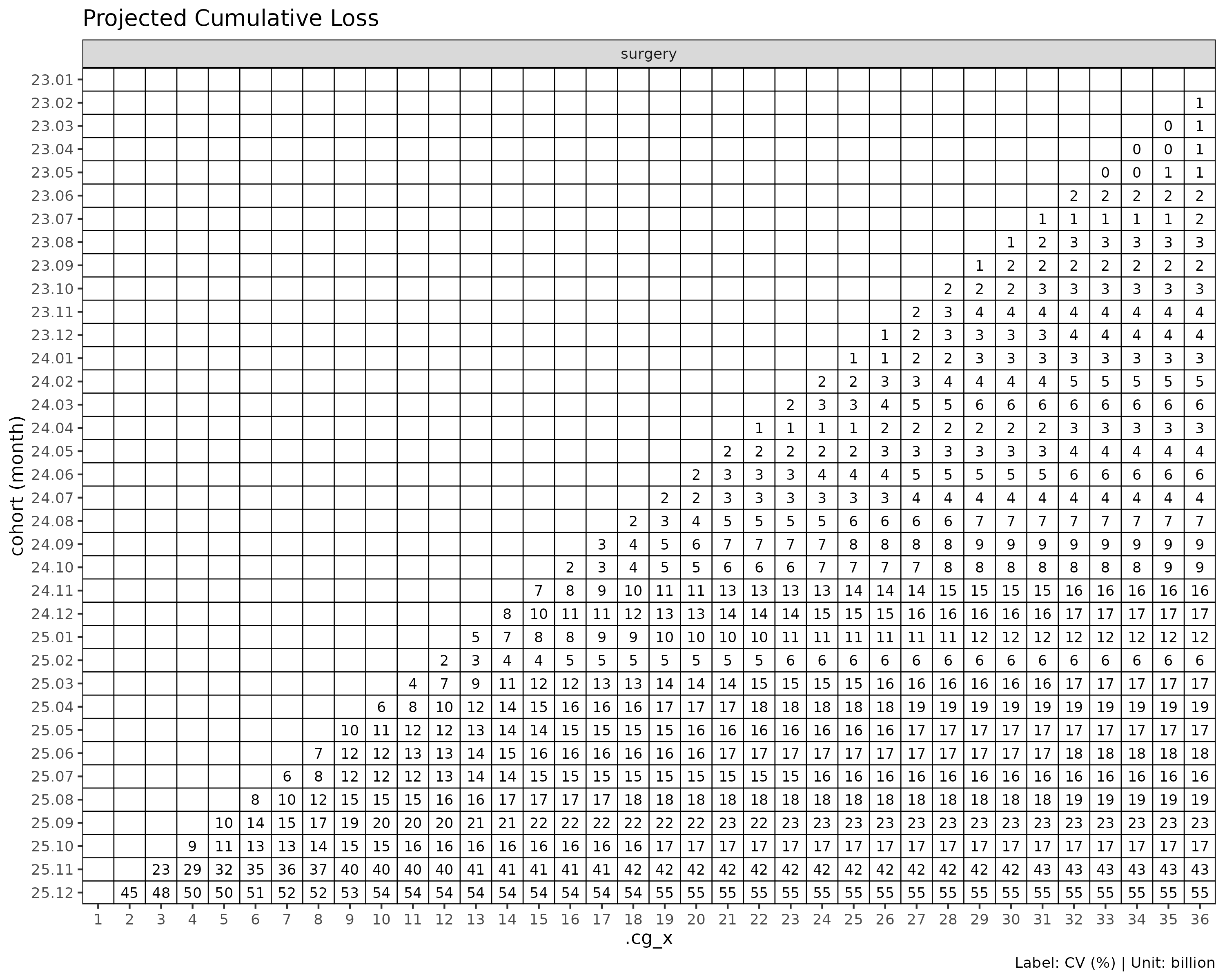
The label_style argument of plot_triangle()
switches the cell labels between value ("value"),
coefficient of variation ("cv"), standard error
("se"), and confidence interval ("ci"). For
the detailed arguments of plot() – type,
region, and so on – see each class’s help page
(?plot.CLFit and friends).
The CL / ED / SA / BF / CC / premium fit results all support
plot() and plot_triangle() the same way, so
the visualisation interface is identical regardless of method.
See also
This tutorial follows the core workflow in one pass. For the methodological background and detailed options of each topic, see:
-
?as_triangle,?fit_cl,?fit_sa,?fit_ratioand other per-function help pages. -
vignette("projection")– projection methods in depth. -
vignette("diagnostics")– maturity, convergence, and regime detection. -
vignette("backtest")– the validation procedure. -
vignette("bootstrap-se-decomposition")– bootstrap standard errors and variance decomposition.