Projection methods

Korean version: 예측 방법론

This is a deep-dive into the five projection methods in lossratio — exposure-driven (ED), chain ladder (CL), stage-adaptive (SA), Bornhuetter-Ferguson (BF), and Cape Cod (CC). The getting-started tutorial shows how to call each fit; this document explains why each method exists, what assumption it rests on, and when one is preferable to another. The intended reader is a practitioner working on long-term health insurance loss ratios.

Why a dedicated projection toolkit

Loss ratio is a daily task in long-term health insurance: analysing cohort-level patterns, projecting ultimate outcomes, and monitoring realised experience against expectations. Existing reserving toolkits mostly trace back to property and casualty (P&C) origins, where the following long-term health characteristics are not directly captured:

Denominator effect and inertia — Cumulative loss ratio’s denominator grows mechanically with development, dampening the signal of recent experience.
Recurrent claims — Hospitalisation, surgery (grade 1-5), and outpatient coverage allow a single insured to file multiple claims; cumulative claim count can exceed insured count.
Risk premium decomposition — In Korea, long-term insurance premium splits into risk premium + savings premium + loading premium. The actuarially meaningful denominator for loss ratio is the risk premium portion alone.
Levelled premium — Non-renewable contracts charge a level premium computed at issue as the lifetime average. The charged premium is not premium; the period risk premium (morbidity rate x sum insured x persistency) must be constructed externally before being passed in.
Regime change — Product redesigns, rate revisions, channel-mix shifts, and underwriting updates introduce cohort-level structural breaks in loss-ratio dynamics.

lossratio transplants core P&C reserving methodology — Mack (1993) chain ladder, Bornhuetter-Ferguson (1972), Cape Cod (Stanard 1985), Bühlmann-Straub (1970) credibility, and Sherman (1984) tail extrapolation — and adapts each piece to the long-term health issues above. The academic lineage is preserved; the goal is a tool that domain practitioners can use immediately.

Methodological lineage

The methodological roots of long-term loss-ratio estimation lie in the following P&C reserving thread:

1967  Bühlmann credibility           experience rating formalised
1970  Bühlmann-Straub                premium-varying credibility
                                     (volume-weighted estimator)
1972  Bornhuetter-Ferguson           prior + observed loss blending
1984  Sherman                        chain ladder tail extrapolation
1985  Stanard (Cape Cod)             reserving application of B-S
1993  Mack                           distribution-free MSE for chain
                                     ladder

Two core ideas drive everything that follows:

Chain ladder (Mack 1993) — Markov multiplicative recursion on cumulative loss $C_k$ : $C_{k+1} = f_k \cdot C_k$ where $f_k = \sum_i C_{i,k+1} / \sum_i C_{i,k}$ .
Cape Cod / Bühlmann-Straub — Loss anchored to premium (volume). $\widehat{ELR} = \sum_i L_i / \sum_i \pi_i$ yields a single ratio that drives ultimate estimation.

Both apply partially to long-term health, but both have cracks:

Domain issue	Chain ladder	Cape Cod
Denominator effect / inertia	Early-dev $f_k$ over-volatile (small $C_k$ )	Cohort-level ELR variation ignored
Levelled premium	Loss-only avoids it (weak against incidence shifts)	Flat $\pi$ absorbs developing premium
Recurrent claims	Works (freq x sev decoupled)	Works (volume measure only)
Developing risk premium	Not relevant	Single $\pi$ assumption breaks
Cohort-level regime change	Violates Mack’s no-calendar-year-effect	Cohort heterogeneity averaged out

Chain ladder is weak early; Cape Cod cannot track developing premium. Each paradigm is incomplete on its own — which is exactly why the package offers five methods rather than one.

The core framework: loss / premium / ratio

All estimation rests on three observable quantities:

Quantity	Meaning	Triangle column
loss	Cumulative loss	`loss`, `incr_loss`
premium	Risk-bearing volume (risk premium for long-term health)	`premium`, `incr_premium`
ratio	Loss ratio (cumulative loss / cumulative premium)	`ratio`, `incr_ratio`

All three are stochastic observables developing over the cohort x dev grid. Premium is not a fixed underwriting volume; it is a developing quantity driven by morbidity x sum insured x persistency — the volume measure of Mack (1993), the natural weight of Bühlmann-Straub (1970).

For cohort $i$ at development period $k$ the projection methods use this notation:

$C^L_{i,k}$ — cumulative loss
$C^P_{i,k}$ — cumulative risk premium (premium)
$f_k = C^L_{k+1} / C^L_k$ — age-to-age (chain ladder) factor
$g_k = \Delta C^L_k / C^P_k$ — exposure-driven intensity
maturity point $k^*$ — the development period at which $f_k$ stabilises for a group (detected from CV / RSE thresholds)

We use the surgery group throughout for brevity — every step generalises to multi-group input.

library(lossratio)
data(experience)
tri <- as_triangle(
  experience[coverage == "surgery"],
  groups   = "coverage",
  cohort   = "uy_m",
  calendar = "cy_m",
  loss     = "incr_loss",
  premium  = "incr_premium"
)

Direct estimation: ED, CL, SA

The three direct-estimation methods estimate factors from the data and chain them forward. Their order — ed -> cl -> sa — mirrors the methodological progression primitive (ED) -> classical (CL) -> composition (SA).

Method	Point estimate	Variance helper	Domain character
`"ed"` (default)	$\Delta L_{k+1} = g_k \cdot P_k$ (additive)	`.ed_g_var` (B-S 1970)	Robust to early-dev ATA volatility
`"cl"`	$L_{k+1} = f_k \cdot L_k$ (multiplicative)	`.mack_f_var` (Mack 1993)	Natural after late-dev factor stabilisation
`"sa"`	ED before maturity $k^*$ , CL after	Composition	Stage-adaptive composition of ED and CL

Exposure-driven (`"ed"`, default)

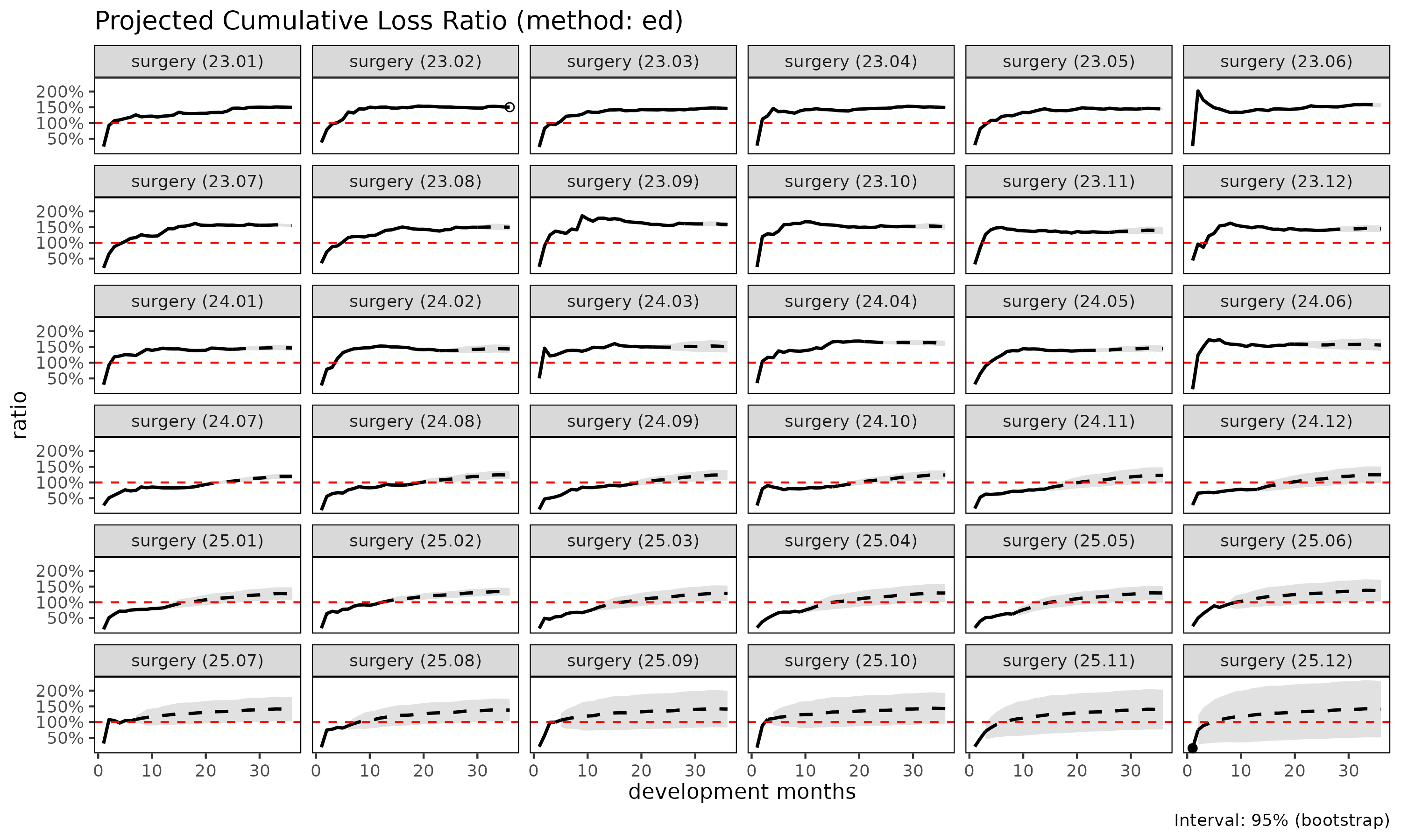
ED projects every future increment using premium (risk premium) as the denominator:

$\hat{C}^L_{i,k+1} = \hat{C}^L_{i,k} + g_k \cdot C^P_{i,k}$

ED is the default because it is an unconditional safe baseline: no maturity or regime detection is required, and the projection is robust under early-dev age-to-age volatility. Because the small $C_k$ of early dev never enters the denominator, ED does not inflate the estimate the way an early $f_k$ can.

The trade-off is cohort homogeneity. The pooled intensity $g_k$ assumes cohorts are reasonably homogeneous in loss-per-premium level. Under cohort-level drift the projection biases toward the pooled mean and may over-project post-change cohorts — see the regime argument for explicit filtering.

When to use ED: as a baseline where cohort homogeneity is plausible; short-tail products where chain ladder offers no advantage; sparse data where age-to-age factors are unreliable across all links.

ratio_ed <- fit_ratio(tri, method = "ed")        # default
plot(ratio_ed, metric = "ratio")

summary(ratio_ed)
#>     coverage     cohort     latest   loss_ult    reserve premium_ult
#>       <char>     <Date>      <num>      <num>      <num>       <num>
#>  1:  surgery 2023-01-01  410248522  410248522          0   274192564
#>  2:  surgery 2023-02-01  976330445 1001304261   24973816   665667720
#>  3:  surgery 2023-03-01  978486045 1027365215   48879170   702047332
#>  4:  surgery 2023-04-01 2029909919 2186835972  156926053  1464399410
#>  5:  surgery 2023-05-01  624219436  700124202   75904766   483147255
#>  6:  surgery 2023-06-01  802880717  924502357  121621640   591568799
#>  7:  surgery 2023-07-01 2539141549 3028986426  489844877  1958263736
#>  8:  surgery 2023-08-01  393678329  488454953   94776624   327535560
#>  9:  surgery 2023-09-01 1364052542 1725804921  361752379  1091733892
#> 10:  surgery 2023-10-01  979266043 1308019740  328753697   864204933
#> 11:  surgery 2023-11-01  604685679  876716310  272030631   630311110
#> 12:  surgery 2023-12-01 1026345366 1527010394  500665028  1057060867
#> 13:  surgery 2024-01-01 1912177598 2942802614 1030625016  2009045340
#> 14:  surgery 2024-02-01  733902485 1193629493  459727008   832229795
#> 15:  surgery 2024-03-01  415459873  685046660  269586787   454345985
#> 16:  surgery 2024-04-01 3286053526 5424401591 2138348065  3372494516
#> 17:  surgery 2024-05-01 1451731153 2740753232 1289022079  1899849125
#> 18:  surgery 2024-06-01  629668308 1170293302  540624994   750125230
#> 19:  surgery 2024-07-01 1250954693 3461664518 2210709825  2891548085
#> 20:  surgery 2024-08-01  425346694 1212435170  787088476   976935246
#> 21:  surgery 2024-09-01  278156543  870725770  592569227   703906575
#> 22:  surgery 2024-10-01  352070323 1217843289  865772966   984833529
#> 23:  surgery 2024-11-01   99050501  398006955  298956454   324081360
#> 24:  surgery 2024-12-01  103194013  456590846  353396833   366444614
#> 25:  surgery 2025-01-01  227089025 1064623873  837534848   833732378
#> 26:  surgery 2025-02-01  939163074 4386331021 3447167947  3286151352
#> 27:  surgery 2025-03-01  112828845  727050149  614221304   566316398
#> 28:  surgery 2025-04-01   82472453  616924302  534451849   476819833
#> 29:  surgery 2025-05-01  141214851 1330756277 1189541426  1027051048
#> 30:  surgery 2025-06-01  136406102 1072907077  936500975   783037474
#> 31:  surgery 2025-07-01  149144024 1209357471 1060213447   859730812
#> 32:  surgery 2025-08-01  116327076 1432029264 1315702188  1037192185
#> 33:  surgery 2025-09-01   67465470  865239645  797774175   611257142
#> 34:  surgery 2025-10-01  121626173 1911124852 1789498679  1338462726
#> 35:  surgery 2025-11-01   15716444  828091909  812375465   593147593
#> 36:  surgery 2025-12-01    4825085 1442904476 1438079391  1022559927
#>     coverage     cohort     latest   loss_ult    reserve premium_ult
#>       <char>     <Date>      <num>      <num>      <num>       <num>
#>     ratio_latest ratio_ult maturity_from loss_proc_se loss_param_se
#>            <num>     <num>         <num>        <num>         <num>
#>  1:    1.4962059  1.496206            NA            0             0
#>  2:    1.5107824  1.504210            NA      2934231       4309793
#>  3:    1.4771448  1.463385            NA      3982661       5158162
#>  4:    1.5139132  1.493333            NA      6546789      11609585
#>  5:    1.4543748  1.449091            NA      4547580       3813039
#>  6:    1.5796369  1.562798            NA     17628088       8903464
#>  7:    1.5597190  1.546771            NA     35686361      31442590
#>  8:    1.4945957  1.491304            NA     16152143       5121110
#>  9:    1.6079808  1.580793            NA     37357117      20421919
#> 10:    1.5129472  1.513553            NA     37573001      17215247
#> 11:    1.3298743  1.390926            NA     35161608      12015326
#> 12:    1.3981081  1.444581            NA     53162531      22167720
#> 13:    1.4274951  1.464777            NA     76259904      44384184
#> 14:    1.3793745  1.434255            NA     51529679      18632983
#> 15:    1.4969280  1.507764            NA     41482939      11326747
#> 16:    1.6712898  1.608424            NA    120195326      95592928
#> 17:    1.3770835  1.442616            NA     88447102      46270702
#> 18:    1.5918247  1.560131            NA     66834389      21472291
#> 19:    0.8658750  1.197167            NA    104028932      46251465
#> 20:    0.9236050  1.241060            NA     62896850      16977280
#> 21:    0.8920448  1.236991            NA     56583751      11941938
#> 22:    0.8596968  1.236598            NA     71133708      16328611
#> 23:    0.7871749  1.228108            NA     41388948       5266012
#> 24:    0.7813438  1.246002            NA     48660596       6215769
#> 25:    0.8188282  1.276937            NA     82549103      15683804
#> 26:    0.9377837  1.334793            NA    193613125      74852479
#> 27:    0.7193486  1.283823            NA     71295313      10069046
#> 28:    0.6947510  1.293831            NA     68826316       8438639
#> 29:    0.6203897  1.295706            NA    116537796      18989499
#> 30:    0.8981587  1.370186            NA    137078933      22543675
#> 31:    1.0440457  1.406670            NA    166193829      31402939
#> 32:    0.8100543  1.380679            NA    184425493      33103273
#> 33:    0.9985960  1.415508            NA    180452022      27168526
#> 34:    1.0894657  1.427851            NA    331672128      79057462
#> 35:    0.4765917  1.396098            NA    190733674      20867271
#> 36:    0.1689836  1.411071            NA    464027946      65288155
#>     ratio_latest ratio_ult maturity_from loss_proc_se loss_param_se
#>            <num>     <num>         <num>        <num>         <num>
#>     loss_total_se loss_total_cv    ratio_se    ratio_cv ratio_ci_lo ratio_ci_hi
#>             <num>         <num>       <num>       <num>       <num>       <num>
#>  1:             0   0.000000000 0.000000000 0.000000000   1.4962059    1.496206
#>  2:       5213830   0.005207039 0.007832482 0.005207039   1.4888589    1.519562
#>  3:       6516765   0.006343182 0.009282515 0.006343182   1.4451911    1.481578
#>  4:      13328275   0.006094776 0.009101530 0.006094776   1.4754943    1.511172
#>  5:       5934623   0.008476529 0.012283260 0.008476529   1.4250160    1.473165
#>  6:      19748953   0.021361712 0.033384034 0.021361712   1.4973662    1.628229
#>  7:      47562095   0.015702314 0.024287890 0.015702314   1.4991681    1.594375
#>  8:      16944542   0.034690081 0.051733442 0.034690081   1.3899079    1.592699
#>  9:      42574746   0.024669501 0.038997366 0.024669501   1.5043592    1.657226
#> 10:      41329107   0.031596700 0.047823272 0.031596700   1.4198208    1.607285
#> 11:      37157863   0.042382995 0.058951622 0.042382995   1.2753833    1.506469
#> 12:      57599154   0.037720211 0.054489912 0.037720211   1.3377831    1.551380
#> 13:      88235644   0.029983541 0.043919190 0.029983541   1.3786966    1.550857
#> 14:      54795036   0.045906235 0.065841233 0.045906235   1.3052083    1.563301
#> 15:      43001505   0.062771643 0.094644843 0.062771643   1.3222638    1.693265
#> 16:     153573839   0.028311665 0.045537165 0.028311665   1.5191729    1.697675
#> 17:      99819176   0.036420344 0.052540580 0.036420344   1.3396386    1.545594
#> 18:      70198966   0.059984079 0.093582996 0.059984079   1.3767113    1.743550
#> 19:     113847340   0.032888034 0.039372453 0.032888034   1.1199979    1.274335
#> 20:      65147845   0.053733055 0.066685940 0.053733055   1.1103579    1.371762
#> 21:      57830189   0.066416077 0.082156058 0.066416077   1.0759676    1.398013
#> 22:      72983751   0.059928689 0.074107704 0.059928689   1.0913497    1.381847
#> 23:      41722607   0.104828839 0.128741150 0.104828839   0.9757801    1.480436
#> 24:      49055982   0.107439697 0.133870114 0.107439697   0.9836217    1.508383
#> 25:      84025806   0.078925344 0.100782707 0.078925344   1.0794067    1.474468
#> 26:     207578746   0.047324004 0.063167737 0.047324004   1.2109863    1.458599
#> 27:      72002829   0.099034199 0.127142405 0.099034199   1.0346287    1.533018
#> 28:      69341707   0.112399053 0.145425384 0.112399053   1.0088025    1.578860
#> 29:     118074803   0.088727594 0.114964882 0.088727594   1.0703790    1.521033
#> 30:     138920305   0.129480276 0.177412077 0.129480276   1.0224648    1.717907
#> 31:     169134660   0.139854976 0.196729788 0.139854976   1.0210866    1.792253
#> 32:     187372862   0.130844297 0.180653947 0.130844297   1.0266036    1.734754
#> 33:     182485783   0.210907792 0.298541761 0.210907792   0.8303773    2.000640
#> 34:     340964049   0.178410138 0.254743029 0.178410138   0.9285635    1.927138
#> 35:     191871774   0.231703476 0.323480658 0.231703476   0.7620871    2.030108
#> 36:     468598419   0.324760527 0.458260104 0.324760527   0.5128975    2.309244
#>     loss_total_se loss_total_cv    ratio_se    ratio_cv ratio_ci_lo ratio_ci_hi
#>             <num>         <num>       <num>       <num>       <num>       <num>

Classical chain ladder (`"cl"`)

CL is the classical Mack (1993) model:

$\hat{C}^L_{i,k+1} = f_k \cdot \hat{C}^L_{i,k}$

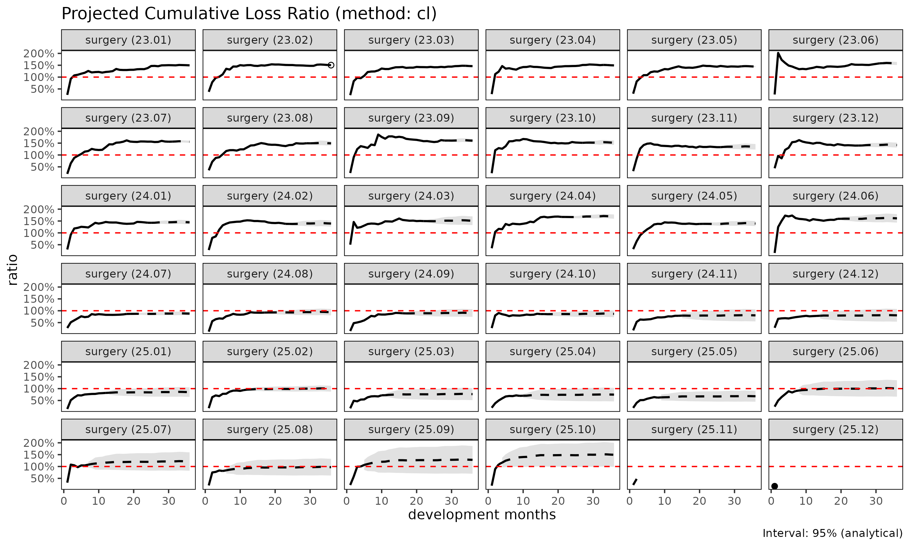
The cohort’s own cumulative loss acts as the anchor, so cohort-level drift propagates naturally without explicit regime detection. The trade-off is the mirror image of ED’s: CL is volatile when early $f_k$ are noisy, because small denominators amplify link errors.

Within fit_ratio(), the CL method projects loss and premium forward — each via chain ladder on its own column — and computes the loss-ratio uncertainty via the delta method. The loss lane alone is equivalent to fit_cl(tri).

When to use CL: once age-to-age factors stabilise; cohort-level drift scenarios where the cohort’s observed trajectory should anchor the projection; reserving exercises where regulators expect the classical Mack form for documentation.

ratio_cl <- fit_ratio(tri, method = "cl")
plot(ratio_cl, metric = "ratio")

Stage-adaptive (`"sa"`)

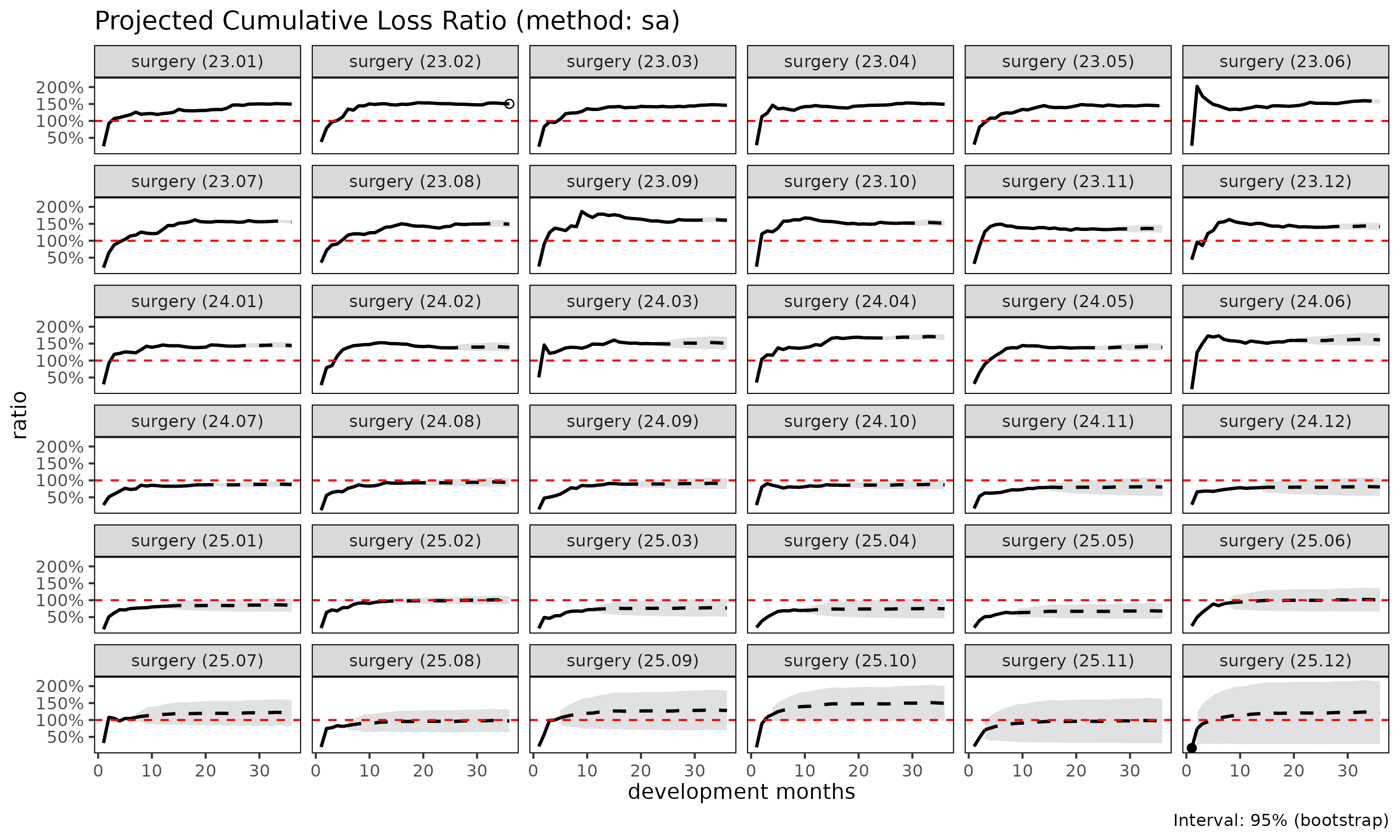
SA composes ED before the maturity point with CL after, exploiting the fact that $f_k$ is volatile early and stable late, while $g_k$ behaves the opposite way:

$\hat{C}^L_{i,k+1} \;=\; \begin{cases} \hat{C}^L_{i,k} + g_k \cdot C^P_{i,k} & k < k^* \quad \text{(ED before maturity)} \\ f_k \cdot \hat{C}^L_{i,k} & k \ge k^* \quad \text{(CL after maturity)} \end{cases}$

Before maturity SA anchors the loss estimate to premium volume, avoiding the volatile-link explosion that classical CL suffers when early $f_k$ are noisy.
After maturity SA preserves the cohort’s own observed level, avoiding the “all cohorts converge to the average” behaviour that pure ED suffers in the tail.

When to use SA: long-tail portfolios where early dev is volatile (ED phase) and cohort-level drift needs cohort-anchored projection in later dev (CL phase); recent cohorts (immature data) mixed with older cohorts (matured); health insurance cohorts with a structural pre-/post-maturity difference (e.g. waiting-period transitions).

ratio_sa <- fit_ratio(tri, method = "sa")
plot(ratio_sa, metric = "ratio")

summary(ratio_sa)
#>     coverage     cohort     latest   loss_ult    reserve premium_ult
#>       <char>     <Date>      <num>      <num>      <num>       <num>
#>  1:  surgery 2023-01-01  410248522  410248522          0   274192564
#>  2:  surgery 2023-02-01  976330445 1001441303   25110858   665667720
#>  3:  surgery 2023-03-01  978486045 1026151243   47665198   702047332
#>  4:  surgery 2023-04-01 2029909919 2186771221  156861302  1464399410
#>  5:  surgery 2023-05-01  624219436  697669301   73449865   483147255
#>  6:  surgery 2023-06-01  802880717  931393934  128513217   591568799
#>  7:  surgery 2023-07-01 2539141549 3050990158  511848609  1958263736
#>  8:  surgery 2023-08-01  393678329  488218204   94539875   327535560
#>  9:  surgery 2023-09-01 1364052542 1751869308  387816766  1091733892
#> 10:  surgery 2023-10-01  979266043 1311793843  332527800   864204933
#> 11:  surgery 2023-11-01  604685679  848103123  243417444   630311110
#> 12:  surgery 2023-12-01 1026345366 1497869029  471523663  1057060867
#> 13:  surgery 2024-01-01 1912177598 2901492851  989315253  2009045340
#> 14:  surgery 2024-02-01  733902485 1160045952  426143467   832229795
#> 15:  surgery 2024-03-01  415459873  686574148  271114275   454345985
#> 16:  surgery 2024-04-01 3286053526 5687484014 2401430488  3372494516
#> 17:  surgery 2024-05-01 1451731153 2645801838 1194070685  1899849125
#> 18:  surgery 2024-06-01  629668308 1209024555  579356247   750125230
#> 19:  surgery 2024-07-01 1250954693 2542927190 1291972497  2891548085
#> 20:  surgery 2024-08-01  425346694  918120582  492773888   976935246
#> 21:  surgery 2024-09-01  278156543  635470028  357313485   703906575
#> 22:  surgery 2024-10-01  352070323  856446521  504376198   984833529
#> 23:  surgery 2024-11-01   99050501  260916096  161865595   324081360
#> 24:  surgery 2024-12-01  103194013  295637296  192443283   366444614
#> 25:  surgery 2025-01-01  227089025  710560093  483471068   833732378
#> 26:  surgery 2025-02-01  939163074 3276849152 2337686078  3286151352
#> 27:  surgery 2025-03-01  112828845  434950057  322121212   566316398
#> 28:  surgery 2025-04-01   82472453  356301148  273828695   476819833
#> 29:  surgery 2025-05-01  141214851  697290587  556075736  1027051048
#> 30:  surgery 2025-06-01  136406102  789468799  653062697   783037474
#> 31:  surgery 2025-07-01  149144024 1040451732  891307708   859730812
#> 32:  surgery 2025-08-01  116327076 1008356733  892029657  1037192185
#> 33:  surgery 2025-09-01   67465470  783000257  715534787   611257142
#> 34:  surgery 2025-10-01  121626173 2001214863 1879588690  1338462726
#> 35:  surgery 2025-11-01   15716444  576954661  561238217   593147593
#> 36:  surgery 2025-12-01    4825085 1246569307 1241744222  1022559927
#>     coverage     cohort     latest   loss_ult    reserve premium_ult
#>       <char>     <Date>      <num>      <num>      <num>       <num>
#>     ratio_latest ratio_ult maturity_from loss_proc_se loss_param_se
#>            <num>     <num>         <num>        <num>         <num>
#>  1:    1.4962059 1.4962059             4            0             0
#>  2:    1.5107824 1.5044162             4      2838052       4263874
#>  3:    1.4771448 1.4616554             4      3880367       4840717
#>  4:    1.5139132 1.4932888             4      7135821      10972855
#>  5:    1.4543748 1.4440097             4      4646457       3580792
#>  6:    1.5796369 1.5744474             4     17348955       8670204
#>  7:    1.5597190 1.5580078             4     38013946      29987964
#>  8:    1.4945957 1.4905808             4     16303418       4959278
#>  9:    1.6079808 1.6046670             4     37742856      20054538
#> 10:    1.5129472 1.5179199             4     39387794      16559819
#> 11:    1.3298743 1.3455310             4     34650050      11722778
#> 12:    1.3981081 1.4170130             4     51946833      22082843
#> 13:    1.4274951 1.4442147             4     73730102      44277226
#> 14:    1.3793745 1.3939010             4     51235927      18527296
#> 15:    1.4969280 1.5111263             4     41831046      11113922
#> 16:    1.6712898 1.6864324             4    118856877      94000634
#> 17:    1.3770835 1.3926379             4     90510561      45996854
#> 18:    1.5918247 1.6117636             4     66688102      21223812
#> 19:    0.8658750 0.8794345             4    104142855      46376952
#> 20:    0.9236050 0.9397968             4     62641056      17014220
#> 21:    0.8920448 0.9027761             4     56889317      11861881
#> 22:    0.8596968 0.8696358             4     67281634      16371282
#> 23:    0.7871749 0.8050944             4     43610819       5306326
#> 24:    0.7813438 0.8067721             4     49362868       6380942
#> 25:    0.8188282 0.8522640             4     81647027      16077360
#> 26:    0.9377837 0.9971693             4    184888599      76955907
#> 27:    0.7193486 0.7680337             4     73183198      10391123
#> 28:    0.6947510 0.7472448             4     68965019       8663440
#> 29:    0.6203897 0.6789250             4    117297078      19478869
#> 30:    0.8981587 1.0082133             4    134689808      23300101
#> 31:    1.0440457 1.2102064             4    164702068      31947996
#> 32:    0.8100543 0.9721985             4    174053848      34060502
#> 33:    0.9985960 1.2809670             4    180505913      28824273
#> 34:    1.0894657 1.4951592             4    341752123      82043614
#> 35:    0.4765917 0.9727000             4    198381074      21884900
#> 36:    0.1689836 1.2190672             4    480416590      66092613
#>     ratio_latest ratio_ult maturity_from loss_proc_se loss_param_se
#>            <num>     <num>         <num>        <num>         <num>
#>     loss_total_se loss_total_cv    ratio_se    ratio_cv ratio_ci_lo ratio_ci_hi
#>             <num>         <num>       <num>       <num>       <num>       <num>
#>  1:             0   0.000000000 0.000000000 0.000000000   1.4962059   1.4962059
#>  2:       5122027   0.005114655 0.007694570 0.005114655   1.4893351   1.5194973
#>  3:       6204014   0.006045906 0.008837031 0.006045906   1.4443351   1.4789756
#>  4:      13089060   0.005985564 0.008938176 0.005985564   1.4757703   1.5108073
#>  5:       5866144   0.008408201 0.012141523 0.008408201   1.4202127   1.4678066
#>  6:      19394810   0.020823424 0.032785384 0.020823424   1.5101892   1.6387055
#>  7:      48418365   0.015869722 0.024725150 0.015869722   1.5095474   1.6064682
#>  8:      17041006   0.034904487 0.052027956 0.034904487   1.3886078   1.5925537
#>  9:      42740001   0.024396798 0.039148735 0.024396798   1.5279369   1.6813971
#> 10:      42727344   0.032571691 0.049441217 0.032571691   1.4210169   1.6148229
#> 11:      36579359   0.043130792 0.058033816 0.043130792   1.2317868   1.4592752
#> 12:      56445774   0.037684052 0.053398793 0.037684052   1.3123533   1.5216727
#> 13:      86003492   0.029641118 0.042808139 0.029641118   1.3603123   1.5281171
#> 14:      54482850   0.046966114 0.065466113 0.046966114   1.2655898   1.5222122
#> 15:      43282278   0.063040938 0.095262817 0.063040938   1.3244146   1.6978379
#> 16:     151535726   0.026643719 0.044932831 0.026643719   1.5983657   1.7744991
#> 17:     101527692   0.038373128 0.053439871 0.038373128   1.2878976   1.4973781
#> 18:      69983949   0.057884638 0.093296354 0.057884638   1.4289061   1.7946211
#> 19:     114002439   0.044831185 0.039426091 0.044831185   0.8021608   0.9567082
#> 20:      64910597   0.070699425 0.066443091 0.070699425   0.8095707   1.0700228
#> 21:      58112809   0.091448544 0.082557560 0.091448544   0.7409662   1.0645859
#> 22:      69244762   0.080851239 0.070311134 0.080851239   0.7318285   1.0074431
#> 23:      43932455   0.168377712 0.135559957 0.168377712   0.5394018   1.0707871
#> 24:      49773579   0.168360283 0.135828381 0.168360283   0.5405534   1.0729908
#> 25:      83214894   0.117111691 0.099810079 0.117111691   0.6566398   1.0478882
#> 26:     200264839   0.061115062 0.060942062 0.061115062   0.8777250   1.1166135
#> 27:      73917223   0.169944163 0.130522838 0.169944163   0.5122136   1.0238537
#> 28:      69507043   0.195079480 0.145772130 0.195079480   0.4615367   1.0329529
#> 29:     118903452   0.170522095 0.115771706 0.170522095   0.4520166   0.9058333
#> 30:     136690304   0.173142123 0.174564192 0.173142123   0.6660738   1.3503528
#> 31:     167772005   0.161249196 0.195144809 0.161249196   0.8277296   1.5926832
#> 32:     177355179   0.175885353 0.170995484 0.175885353   0.6370536   1.3073435
#> 33:     182792843   0.233451830 0.299044102 0.233451830   0.6948514   1.8670827
#> 34:     351462186   0.175624413 0.262586457 0.175624413   0.9804992   2.0098192
#> 35:     199584567   0.345927644 0.336483818 0.345927644   0.3132038   1.6321962
#> 36:     484941577   0.389020951 0.474242696 0.389020951   0.2895686   2.1485658
#>     loss_total_se loss_total_cv    ratio_se    ratio_cv ratio_ci_lo ratio_ci_hi
#>             <num>         <num>       <num>       <num>       <num>       <num>

Comparing ED, CL, SA

ratios <- list(
  ed = fit_ratio(tri, method = "ed"),
  cl = fit_ratio(tri, method = "cl"),
  sa = fit_ratio(tri, method = "sa")
)

# Cohort-level ultimate-loss summary
summary(ratios$ed)$loss_ult
#>  [1]  410248522 1001304261 1027365215 2186835972  700124202  924502357
#>  [7] 3028986426  488454953 1725804921 1308019740  876716310 1527010394
#> [13] 2942802614 1193629493  685046660 5424401591 2740753232 1170293302
#> [19] 3461664518 1212435170  870725770 1217843289  398006955  456590846
#> [25] 1064623873 4386331021  727050149  616924302 1330756277 1072907077
#> [31] 1209357471 1432029264  865239645 1911124852  828091909 1442904476
summary(ratios$cl)$loss_ult
#>  [1]  410248522 1001441303 1026151243 2186771221  697669301  931393934
#>  [7] 3050990158  488218204 1751869308 1311793843  848103123 1497869029
#> [13] 2901492851 1160045952  686574148 5687484014 2645801838 1209024555
#> [19] 2542927190  918120582  635470028  856446521  260916096  295637296
#> [25]  710560093 3276849152  434950057  356301148  697290587  789468799
#> [31] 1040451732 1008356733  783000257 2001214863         NA         NA
summary(ratios$sa)$loss_ult
#>  [1]  410248522 1001441303 1026151243 2186771221  697669301  931393934
#>  [7] 3050990158  488218204 1751869308 1311793843  848103123 1497869029
#> [13] 2901492851 1160045952  686574148 5687484014 2645801838 1209024555
#> [19] 2542927190  918120582  635470028  856446521  260916096  295637296
#> [25]  710560093 3276849152  434950057  356301148  697290587  789468799
#> [31] 1040451732 1008356733  783000257 2001214863  576954661 1246569307

Method	Mechanism	When to use
ED	pooled $g_k$ x cohort premium	default baseline; assumes cohort homogeneity
CL	pooled $f_k$ x cohort cum_loss	cohort-level drift; cohort-anchored
SA	ED early + CL late	long-tail with both volatile early dev and cohort-level late drift

Prior-anchored estimation: BF and CC

ED, CL, and SA all estimate factors from the data. When the observed triangle is thin — immature cohorts, or cohorts right after a rate change — that estimate can be unstable. The prior-anchored family blends an expected loss ratio (ELR) with whatever loss has already emerged:

$\text{Ult} = L_{\text{latest}} + \left(1 - \tfrac{1}{\text{LDF}}\right) \cdot \pi \cdot \text{ELR}$

The two methods differ only in where the ELR comes from.

Method	ELR source	Domain use case
`"bf"`	External (user supplied via `prior`)	Immature and post-rate-change cohorts — anchor on an external prior when observed data is thin (Bornhuetter-Ferguson 1972)
`"cc"`	Derived from data (payout-weighted $\sum L / \sum \pi \cdot \text{payout}$ )	Cohort-cohesive estimation — when pricing/industry suggests a natural single ELR target (Stanard 1985, Cape Cod)

Bornhuetter-Ferguson (`"bf"`)

BF takes the ELR as an external input. The emerged loss $L_{\text{latest}}$ is kept as-is, and only the unemerged portion $(1 - 1/\text{LDF})$ is filled in from the prior. As a cohort matures the data term dominates and the prior fades — BF degrades gracefully toward a chain-ladder answer.

fit_bf(tri, prior = 0.7)
#> <BFFit>
#> method        : bf 
#> loss          : loss 
#> premium       : premium 
#> alpha         : 1 
#> sigma_method  : locf 
#> recent        : all 
#> regime        : none
#> groups        : coverage 
#> cohorts (n)   : 36 
#> prior         : scalar elr = 0.7 
#> ci_type       : analytical

The prior argument also accepts a per-group data.frame, optionally carrying an elr_se column to treat the prior as a distribution rather than a fixed point.

Cape Cod (`"cc"`)

CC has the same blending form as BF but estimates the ELR from the data itself — a payout-weighted pooled ratio across cohorts. It is the natural choice when pricing or industry context suggests a single coherent ELR target and no external prior is on hand.

fit_cc(tri)
#> <CCFit>
#> method        : cc 
#> loss          : loss 
#> premium       : premium 
#> alpha         : 1 
#> sigma_method  : locf 
#> recent        : all 
#> regime        : none
#> groups        : coverage 
#> cohorts (n)   : 36 
#> pooled ELR    :
#>   surgery : 1.3558
#> ci_type       : analytical

Three aggregation axes

ED, CC, and BF differ in how they aggregate the loss-per-premium signal:

ED — per-link $g_k$ : dev-granular, cohort-uniform per link.
CC — cohort-level single ELR: cohort-uniform, dev-aggregated.
BF — external prior: bypasses data estimation altogether.

Together the five methods reconstruct the P&C reserving trinity for long-term health, and the three aggregation axes each serve a distinct use case.

Chain ladder as a reserving worker

fit_cl() is the dedicated chain ladder fit for a single value column. Unlike fit_ratio() — which projects loss and premium jointly to get loss ratio — fit_cl() projects one cumulative metric forward and computes Mack-style standard errors per cohort. This is the classical P&C reserving use case: projecting ultimate paid / incurred loss for an open accident year. Practitioners with a P&C background will recognise the Mack workflow directly.

cl <- fit_cl(tri)
print(cl)
#> <CLFit>
#> method      : mack 
#> loss        : loss 
#> weight      : none 
#> alpha       : 1 
#> sigma_method: locf 
#> recent      : all 
#> regime      : none
#> use_maturity: FALSE 
#> tail_factor : 1 
#> groups      : coverage 
#> periods     : 36

fit_cl() summarises adjacent development links by age-to-age factors $f_k = C^L_{k+1} / C^L_k$ , selected per link and then chained to project each cohort forward to ultimate. On top of the point projection, Mack’s formulae decompose the prediction variance into process and parameter components:

loss_proc_se — process variance, from $\sigma^2_k$ (residual link variance per development period).
loss_param_se — parameter variance, from the uncertainty of the selected age-to-age factors $\hat{f}_k$ .
loss_total_se — total standard error, $\sqrt{\text{loss\_proc\_se}^2 + \text{loss\_param\_se}^2}$ .
loss_total_cv — coefficient of variation, loss_total_se / loss_proj.

summary(cl)
#>     coverage     cohort     latest   loss_ult    reserve loss_proc_se
#>       <char>     <Date>      <num>      <num>      <num>        <num>
#>  1:  surgery 2023-01-01  410248522  410248522          0            0
#>  2:  surgery 2023-02-01  976330445 1001441303   25110858      2751819
#>  3:  surgery 2023-03-01  978486045 1026151243   47665198      3967869
#>  4:  surgery 2023-04-01 2029909919 2186771221  156861302      6942937
#>  5:  surgery 2023-05-01  624219436  697669301   73449865      4455636
#>  6:  surgery 2023-06-01  802880717  931393934  128513217     17869565
#>  7:  surgery 2023-07-01 2539141549 3050990158  511848609     35918003
#>  8:  surgery 2023-08-01  393678329  488218204   94539875     15583801
#>  9:  surgery 2023-09-01 1364052542 1751869308  387816766     38001618
#> 10:  surgery 2023-10-01  979266043 1311793843  332527800     38496097
#> 11:  surgery 2023-11-01  604685679  848103123  243417444     35719579
#> 12:  surgery 2023-12-01 1026345366 1497869029  471523663     51405333
#> 13:  surgery 2024-01-01 1912177598 2901492851  989315253     75674312
#> 14:  surgery 2024-02-01  733902485 1160045952  426143467     51719398
#> 15:  surgery 2024-03-01  415459873  686574148  271114275     41313266
#> 16:  surgery 2024-04-01 3286053526 5687484014 2401430488    122770258
#> 17:  surgery 2024-05-01 1451731153 2645801838 1194070685     93024106
#> 18:  surgery 2024-06-01  629668308 1209024555  579356247     65346187
#> 19:  surgery 2024-07-01 1250954693 2542927190 1291972497    103136528
#> 20:  surgery 2024-08-01  425346694  918120582  492773888     65317866
#> 21:  surgery 2024-09-01  278156543  635470028  357313485     56737053
#> 22:  surgery 2024-10-01  352070323  856446521  504376198     68091257
#> 23:  surgery 2024-11-01   99050501  260916096  161865595     41787166
#> 24:  surgery 2024-12-01  103194013  295637296  192443283     49617195
#> 25:  surgery 2025-01-01  227089025  710560093  483471068     83635489
#> 26:  surgery 2025-02-01  939163074 3276849152 2337686078    192418633
#> 27:  surgery 2025-03-01  112828845  434950057  322121212     72345359
#> 28:  surgery 2025-04-01   82472453  356301148  273828695     68974257
#> 29:  surgery 2025-05-01  141214851  697290587  556075736    119238986
#> 30:  surgery 2025-06-01  136406102  789468799  653062697    136628652
#> 31:  surgery 2025-07-01  149144024 1040451732  891307708    167039609
#> 32:  surgery 2025-08-01  116327076 1008356733  892029657    183653360
#> 33:  surgery 2025-09-01   67465470  783000257  715534787    179947037
#> 34:  surgery 2025-10-01  121626173 2001214863 1879588690    337103186
#> 35:  surgery 2025-11-01   15716444  449653406  433936962    194100658
#> 36:  surgery 2025-12-01    4825085  850839118  846014033    472741759
#>     coverage     cohort     latest   loss_ult    reserve loss_proc_se
#>       <char>     <Date>      <num>      <num>      <num>        <num>
#>     loss_param_se loss_total_se loss_total_cv
#>             <num>         <num>         <num>
#>  1:             0             0   0.000000000
#>  2:       4299412       5104650   0.005097304
#>  3:       5021196       6399718   0.006236623
#>  4:      11297887      13260717   0.006064062
#>  5:       3696918       5789637   0.008298541
#>  6:       8694892      19872657   0.021336469
#>  7:      30501066      47121311   0.015444596
#>  8:       5072721      16388635   0.033568259
#>  9:      20827314      43334744   0.024736288
#> 10:      16992221      42079509   0.032077837
#> 11:      11901733      37650227   0.044393454
#> 12:      22008504      55918535   0.037332059
#> 13:      43971810      87522121   0.030164514
#> 14:      18269127      54851227   0.047283667
#> 15:      11014493      42756344   0.062274911
#> 16:      92689755     153830838   0.027047256
#> 17:      45040851     103354548   0.039063601
#> 18:      20907249      68609309   0.056747655
#> 19:      45568404     112754702   0.044340515
#> 20:      16819267      67448584   0.073463753
#> 21:      11859688      57963310   0.091213288
#> 22:      16219631      69996398   0.081728860
#> 23:       5190764      42108328   0.161386470
#> 24:       6221683      50005754   0.169145620
#> 25:      15668260      85090478   0.119751276
#> 26:      75222224     206599403   0.063048188
#> 27:      10161412      73055495   0.167962950
#> 28:       8575343      69505285   0.195074548
#> 29:      19174475     120770842   0.173200161
#> 30:      22834478     138523651   0.175464377
#> 31:      31445935     169973756   0.163365345
#> 32:      32987225     186592373   0.185045993
#> 33:      27713231     182068556   0.232526816
#> 34:      80113491     346492034   0.173140846
#> 35:      21034520     195237078   0.434194593
#> 36:      66075497     477337136   0.561019265
#>     loss_param_se loss_total_se loss_total_cv
#>             <num>         <num>         <num>
plot(cl, type = "projection", show_interval = TRUE)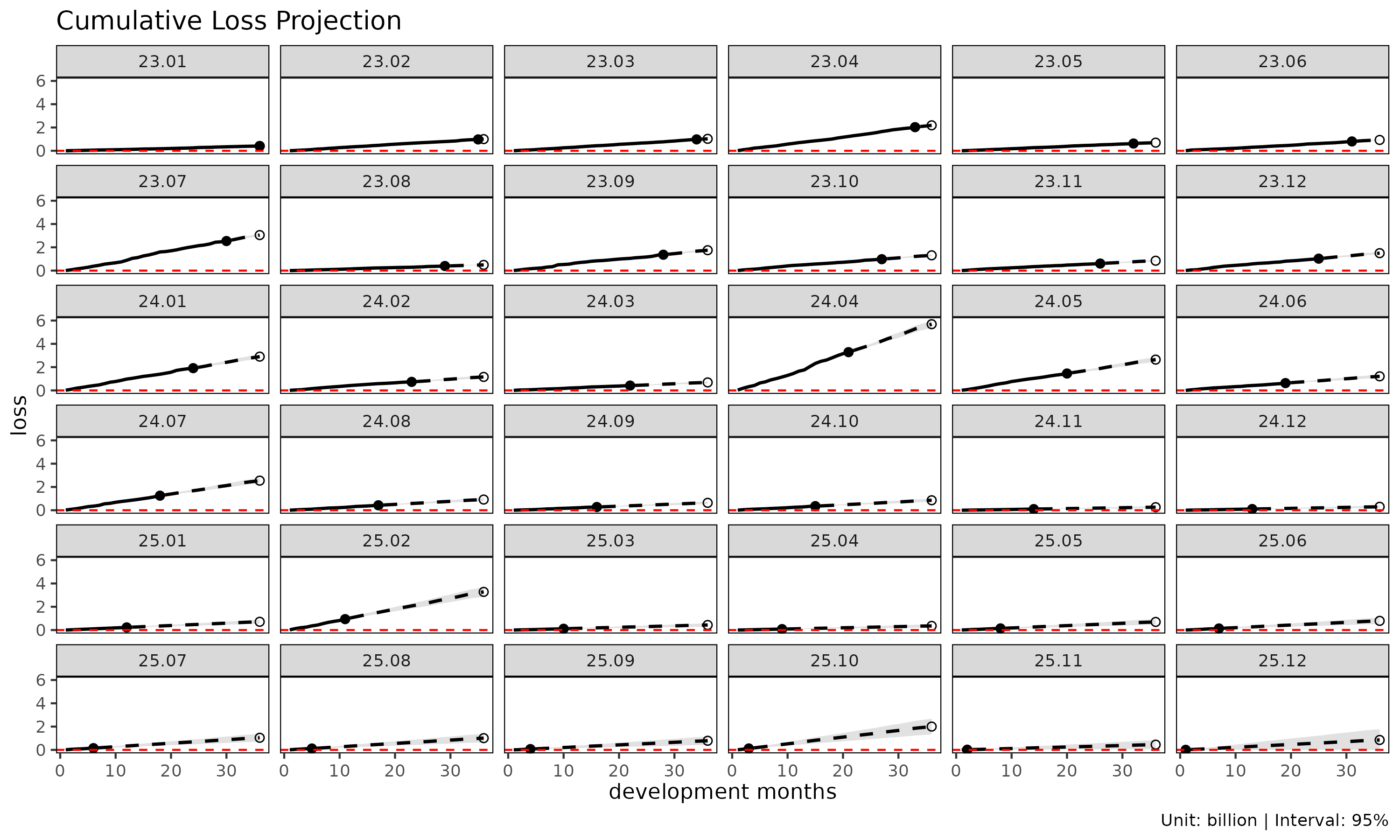

plot(cl, type = "reserve", conf_level = 0.95)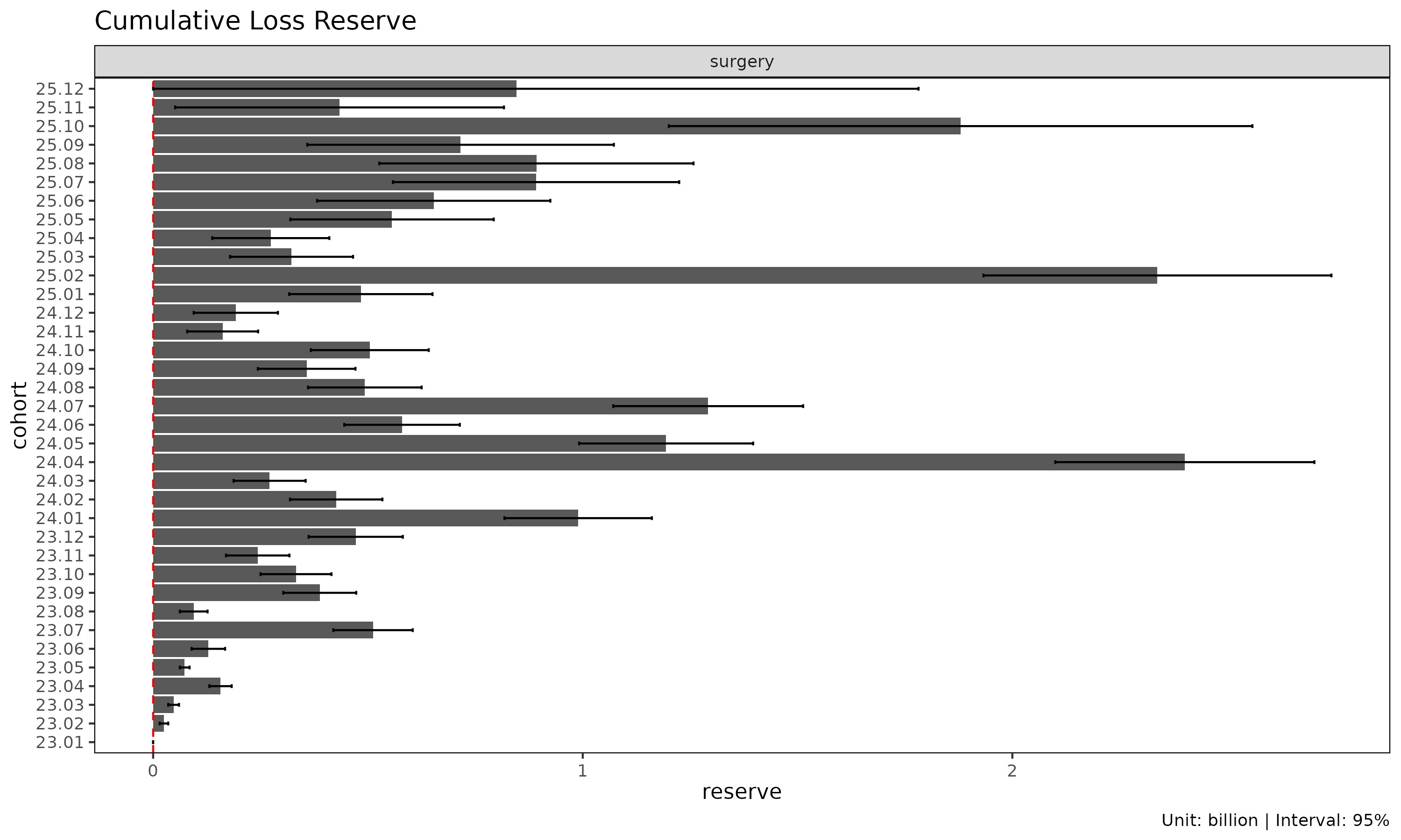

plot_triangle() displays the cohort x dev cells as a heatmap, distinguishing observed cells from projected, with label_style showing per-cell CV / SE / CI:

plot_triangle(cl, region = "full")        # observed + projected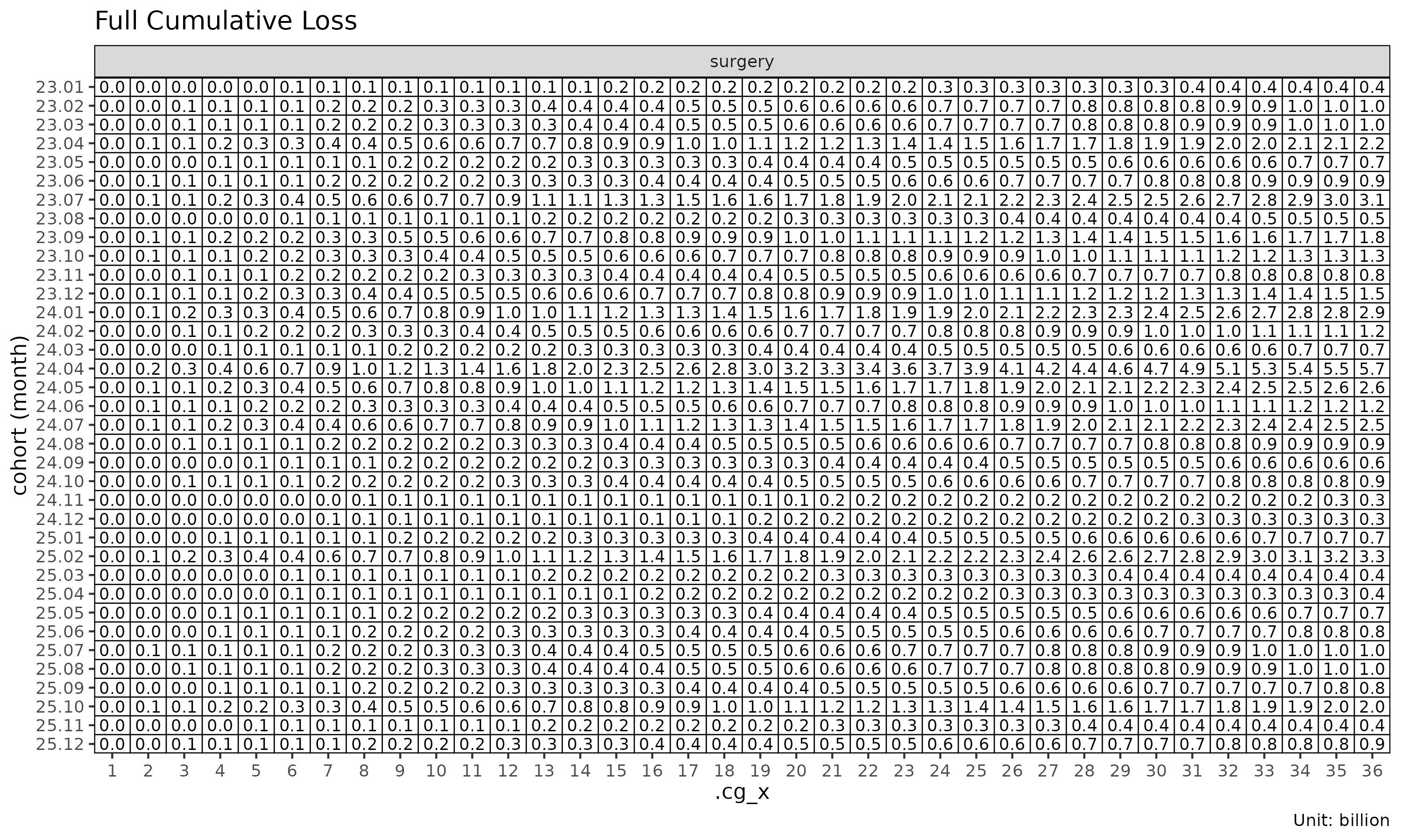

plot_triangle(cl, label_style = "cv")     # per-cell coefficient of variation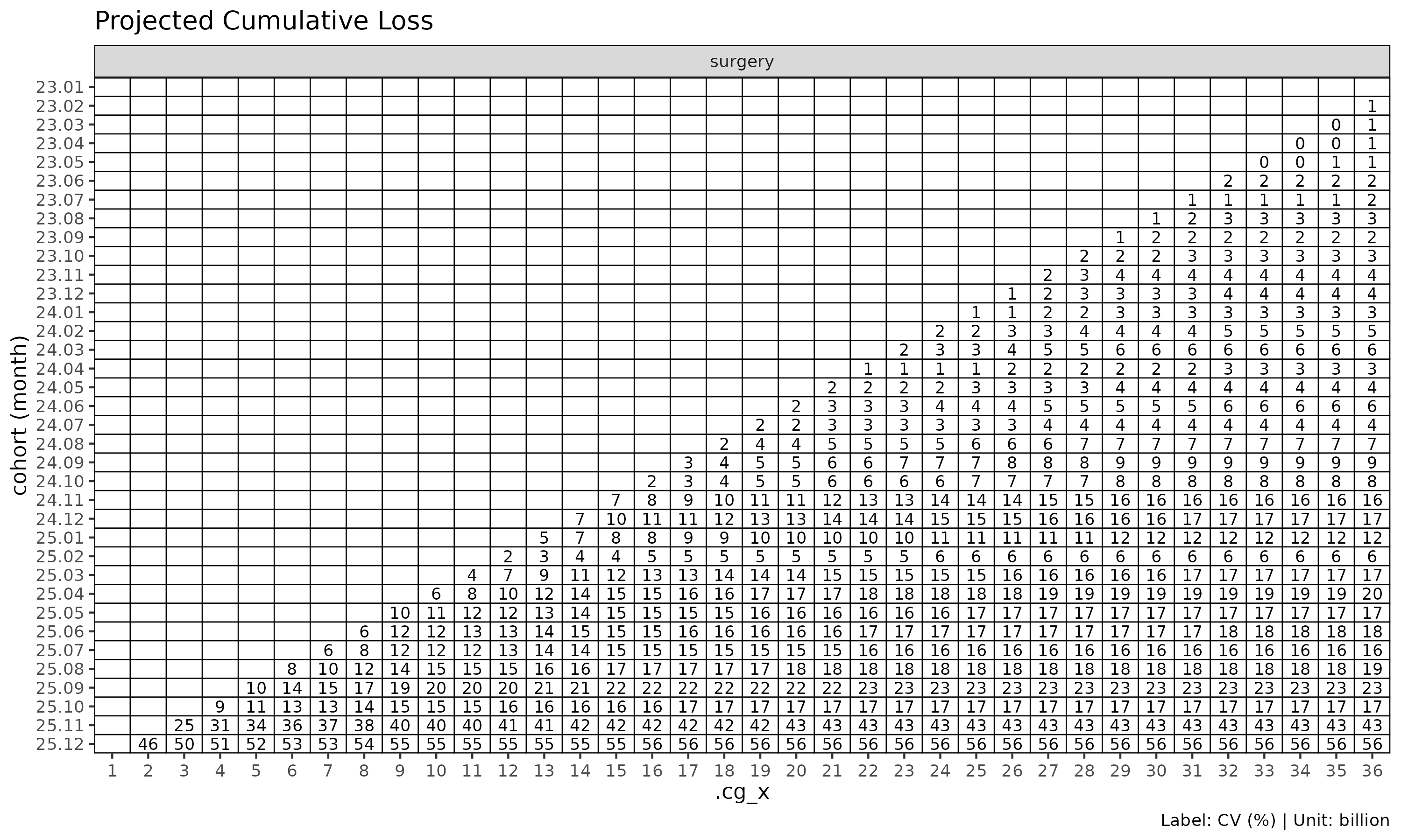

Tail factor

For triangles where the latest observed development period is still developing, an extrapolated tail factor estimates ultimate. The extrapolation fits $\log(f_k - 1) \sim k$ — a Sherman (1984) log-linear tail — to the selected ATA factors and extends the projection by the cumulative product of extrapolated $f_k$ values. Disabled by default (tail = FALSE).

fit_cl(tri, tail = TRUE)         # log-linear extrapolation
#> <CLFit>
#> method      : mack 
#> loss        : loss 
#> weight      : none 
#> alpha       : 1 
#> sigma_method: locf 
#> recent      : all 
#> regime      : none
#> use_maturity: FALSE 
#> tail_factor : 1.188138 
#> groups      : coverage 
#> periods     : 36
fit_cl(tri, tail = 1.025)        # or a literal tail factor
#> <CLFit>
#> method      : mack 
#> loss        : loss 
#> weight      : none 
#> alpha       : 1 
#> sigma_method: locf 
#> recent      : all 
#> regime      : none
#> use_maturity: FALSE 
#> tail_factor : 1.025 
#> groups      : coverage 
#> periods     : 36

Sigma extrapolation methods

Mack variance requires $\sigma_k$ at all development links, including the last where it cannot be estimated directly. sigma_method controls the extrapolation:

`sigma_method`	Behaviour
`"locf"`	(default) last observation carried forward
`"min_last2"`	min of the last two estimable $\sigma$ values — conservative
`"loglinear"`	log-linear extrapolation from the observed $\sigma_k$ sequence
`"mack"`	Mack (1993) Appendix B tail estimator — closed-form for the last link only; LOCF with warning beyond that
`"none"`	no extrapolation; $\sigma$ stays `NA` (variance treated as zero downstream)

fit_cl(tri, sigma_method = "loglinear")
#> <CLFit>
#> method      : mack 
#> loss        : loss 
#> weight      : none 
#> alpha       : 1 
#> sigma_method: loglinear 
#> recent      : all 
#> regime      : none
#> use_maturity: FALSE 
#> tail_factor : 1 
#> groups      : coverage 
#> periods     : 36

Variance and confidence intervals

fit_ratio() reports analytical standard errors for L/P. Two variants control how premium uncertainty enters:

se_method = "fixed" (default) — premium treated as fixed, $\text{SE}(L/P) \approx \text{SE}(L)/P$ . Strictly the delta method with Var(P) = 0 and Cov(L,P) = 0.
se_method = "delta" — full delta method including premium uncertainty and loss-premium correlation rho:

$\mathrm{Var}(L/P) \approx \frac{\mathrm{Var}(L)}{P^2} + \frac{L^2 \mathrm{Var}(P)}{P^4} - \frac{2 \rho L \mathrm{SE}(L) \mathrm{SE}(P)}{P^3}$

There are two complementary paths to SE estimation:

Analytical — .mack_f_var() (Mack 1993) and .ed_g_var() (B-S 1970) provide closed-form per-link variance, distribution-free.
Bootstrap — a residual paradigm (cell / link / parametric) drives forward simulation, capturing distributional shape. Residual choice determines both the process variance scale and the forward-sim model (paradigm matching).

A large divergence between the two paths is a model-misspecification signal; routinely computing both serves as a sanity check.

ratio_boot <- fit_ratio(tri, method = "ed", bootstrap = TRUE,
                        B = 1000, seed = 1)
summary(ratio_boot)
#>     coverage     cohort     latest   loss_ult    reserve premium_ult
#>       <char>     <Date>      <num>      <num>      <num>       <num>
#>  1:  surgery 2023-01-01  410248522  410248522          0   274192564
#>  2:  surgery 2023-02-01  976330445 1001304261   24973816   665667720
#>  3:  surgery 2023-03-01  978486045 1027365215   48879170   702047332
#>  4:  surgery 2023-04-01 2029909919 2186835972  156926053  1464399410
#>  5:  surgery 2023-05-01  624219436  700124202   75904766   483147255
#>  6:  surgery 2023-06-01  802880717  924502357  121621640   591568799
#>  7:  surgery 2023-07-01 2539141549 3028986426  489844877  1958263736
#>  8:  surgery 2023-08-01  393678329  488454953   94776624   327535560
#>  9:  surgery 2023-09-01 1364052542 1725804921  361752379  1091733892
#> 10:  surgery 2023-10-01  979266043 1308019740  328753697   864204933
#> 11:  surgery 2023-11-01  604685679  876716310  272030631   630311110
#> 12:  surgery 2023-12-01 1026345366 1527010394  500665028  1057060867
#> 13:  surgery 2024-01-01 1912177598 2942802614 1030625016  2009045340
#> 14:  surgery 2024-02-01  733902485 1193629493  459727008   832229795
#> 15:  surgery 2024-03-01  415459873  685046660  269586787   454345985
#> 16:  surgery 2024-04-01 3286053526 5424401591 2138348065  3372494516
#> 17:  surgery 2024-05-01 1451731153 2740753232 1289022079  1899849125
#> 18:  surgery 2024-06-01  629668308 1170293302  540624994   750125230
#> 19:  surgery 2024-07-01 1250954693 3461664518 2210709825  2891548085
#> 20:  surgery 2024-08-01  425346694 1212435170  787088476   976935246
#> 21:  surgery 2024-09-01  278156543  870725770  592569227   703906575
#> 22:  surgery 2024-10-01  352070323 1217843289  865772966   984833529
#> 23:  surgery 2024-11-01   99050501  398006955  298956454   324081360
#> 24:  surgery 2024-12-01  103194013  456590846  353396833   366444614
#> 25:  surgery 2025-01-01  227089025 1064623873  837534848   833732378
#> 26:  surgery 2025-02-01  939163074 4386331021 3447167947  3286151352
#> 27:  surgery 2025-03-01  112828845  727050149  614221304   566316398
#> 28:  surgery 2025-04-01   82472453  616924302  534451849   476819833
#> 29:  surgery 2025-05-01  141214851 1330756277 1189541426  1027051048
#> 30:  surgery 2025-06-01  136406102 1072907077  936500975   783037474
#> 31:  surgery 2025-07-01  149144024 1209357471 1060213447   859730812
#> 32:  surgery 2025-08-01  116327076 1432029264 1315702188  1037192185
#> 33:  surgery 2025-09-01   67465470  865239645  797774175   611257142
#> 34:  surgery 2025-10-01  121626173 1911124852 1789498679  1338462726
#> 35:  surgery 2025-11-01   15716444  828091909  812375465   593147593
#> 36:  surgery 2025-12-01    4825085 1442904476 1438079391  1022559927
#>     coverage     cohort     latest   loss_ult    reserve premium_ult
#>       <char>     <Date>      <num>      <num>      <num>       <num>
#>     ratio_latest ratio_ult maturity_from loss_proc_se loss_param_se
#>            <num>     <num>         <num>        <num>         <num>
#>  1:    1.4962059  1.496206            NA            0             0
#>  2:    1.5107824  1.504210            NA      2727872       4252490
#>  3:    1.4771448  1.463385            NA      3857656       4937453
#>  4:    1.5139132  1.493333            NA      6464023      11046456
#>  5:    1.4543748  1.449091            NA      4414172       3642331
#>  6:    1.5796369  1.562798            NA     18256950       8719253
#>  7:    1.5597190  1.546771            NA     36356039      30599176
#>  8:    1.4945957  1.491304            NA     15446049       5099721
#>  9:    1.6079808  1.580793            NA     37907786      20976255
#> 10:    1.5129472  1.513553            NA     39296776      17261695
#> 11:    1.3298743  1.390926            NA     35909652      12014126
#> 12:    1.3981081  1.444581            NA     51167052      22190005
#> 13:    1.4274951  1.464777            NA     73031711      44428929
#> 14:    1.3793745  1.434255            NA     52947591      18568184
#> 15:    1.4969280  1.507764            NA     41658227      11179304
#> 16:    1.6712898  1.608424            NA    125695833      92684211
#> 17:    1.3770835  1.442616            NA     97706383      44982439
#> 18:    1.5918247  1.560131            NA     65035795      20970332
#> 19:    0.8658750  1.197167            NA    106858449      45060454
#> 20:    0.9236050  1.241060            NA     66935131      16625328
#> 21:    0.8920448  1.236991            NA     55505776      11742732
#> 22:    0.8596968  1.236598            NA     67082777      15817555
#> 23:    0.7871749  1.228108            NA     39061897       5053759
#> 24:    0.7813438  1.246002            NA     49219392       6010050
#> 25:    0.8188282  1.276937            NA     84168707      15344194
#> 26:    0.9377837  1.334793            NA    180111087      73529151
#> 27:    0.7193486  1.283823            NA     72550954       9888792
#> 28:    0.6947510  1.293831            NA     66584376       8314150
#> 29:    0.6203897  1.295706            NA    117591452      18442708
#> 30:    0.8981587  1.370186            NA    137403273      22106226
#> 31:    1.0440457  1.406670            NA    171955351      30424127
#> 32:    0.8100543  1.380679            NA    193891884      31690043
#> 33:    0.9985960  1.415508            NA    184974432      26734919
#> 34:    1.0894657  1.427851            NA    322907580      79529875
#> 35:    0.4765917  1.396098            NA    189748454      20768911
#> 36:    0.1689836  1.411071            NA    457843613      67190912
#>     ratio_latest ratio_ult maturity_from loss_proc_se loss_param_se
#>            <num>     <num>         <num>        <num>         <num>
#>     loss_total_se loss_total_cv    ratio_se    ratio_cv ratio_ci_lo ratio_ci_hi
#>             <num>         <num>       <num>       <num>       <num>       <num>
#>  1:             0   0.000000000 0.000000000 0.000000000   1.4962059    1.496206
#>  2:       5052223   0.005045642 0.007589706 0.005045642   1.4893348    1.519086
#>  3:       6265776   0.006098879 0.008925005 0.006098879   1.4458919    1.480877
#>  4:      12798742   0.005852630 0.008739925 0.005852630   1.4762031    1.510463
#>  5:       5722892   0.008174109 0.011845026 0.008174109   1.4258749    1.472307
#>  6:      20232192   0.021884414 0.034200911 0.021884414   1.4957651    1.629830
#>  7:      47519166   0.015688141 0.024265968 0.015688141   1.4992110    1.594332
#>  8:      16266148   0.033301224 0.049662235 0.033301224   1.3939674    1.588640
#>  9:      43324399   0.025103880 0.039684029 0.025103880   1.5030134    1.658572
#> 10:      42920889   0.032813640 0.049665174 0.032813640   1.4162108    1.610895
#> 11:      37866111   0.043190836 0.060075271 0.043190836   1.2731809    1.508672
#> 12:      55771530   0.036523346 0.052760944 0.036523346   1.3411718    1.547991
#> 13:      85484271   0.029048591 0.042549697 0.029048591   1.3813807    1.548172
#> 14:      56109044   0.047007086 0.067420134 0.047007086   1.3021137    1.566396
#> 15:      43132177   0.062962393 0.094932449 0.062962393   1.3217001    1.693828
#> 16:     156172357   0.028790707 0.046307668 0.028790707   1.5176628    1.699186
#> 17:     107563735   0.039246049 0.056616988 0.039246049   1.3316490    1.553584
#> 18:      68333077   0.058389702 0.091095559 0.058389702   1.3815866    1.738675
#> 19:     115970568   0.033501389 0.040106740 0.033501389   1.1185587    1.275774
#> 20:      68968930   0.056884633 0.070597238 0.056884633   1.1026919    1.379428
#> 21:      56734319   0.065157506 0.080599218 0.065157506   1.0790190    1.394962
#> 22:      68922376   0.056593797 0.069983783 0.056593797   1.0994324    1.373764
#> 23:      39387464   0.098961748 0.121535728 0.098961748   0.9899025    1.466314
#> 24:      49584970   0.108598257 0.135313682 0.108598257   0.9807924    1.511212
#> 25:      85555920   0.080362579 0.102617966 0.080362579   1.0758097    1.478065
#> 26:     194541871   0.044351844 0.059200521 0.044351844   1.2187619    1.450824
#> 27:      73221781   0.100710771 0.129294827 0.100710771   1.0304100    1.537236
#> 28:      67101447   0.108767716 0.140727047 0.108767716   1.0180111    1.569651
#> 29:     119028917   0.089444566 0.115893867 0.089444566   1.0685583    1.522854
#> 30:     139170200   0.129713191 0.177731213 0.129713191   1.0218393    1.718533
#> 31:     174626087   0.144395756 0.203117167 0.144395756   1.0085676    1.804772
#> 32:     196464555   0.137193115 0.189419626 0.137193115   1.0094232    1.751934
#> 33:     186896485   0.216005457 0.305757549 0.216005457   0.8162347    2.014782
#> 34:     332557223   0.174011249 0.248462072 0.174011249   0.9408739    1.914827
#> 35:     190881700   0.230507868 0.321811473 0.230507868   0.7653587    2.026836
#> 36:     462747656   0.320705676 0.452538422 0.320705676   0.5241118    2.298030
#>     loss_total_se loss_total_cv    ratio_se    ratio_cv ratio_ci_lo ratio_ci_hi
#>             <num>         <num>       <num>       <num>       <num>       <num>

Maturity input for SA

For method = "sa" the maturity point $k^*$ determines where the projection switches from ED to CL. By default fit_ratio() / fit_loss() use maturity = "auto", which calls detect_maturity() internally with default thresholds. Other forms:

maturity = NULL — disable detection (only meaningful for non-SA methods or for fit_ata() standalone).
maturity = maturity_spec(max_cv = 0.05, min_run = 2L) — a lazy spec forwarding custom thresholds to detect_maturity() at fit time (leakage-safe for backtest()).
maturity = detect_maturity(tri, ...) — a pre-built Maturity object, fixed across refits.
maturity = maturity_at(coverage = "surgery", change = 4) — a manual per-group override (e.g. a company-standard $k^*$ ).

The same lazy-spec / pre-built / manual pattern applies to fit_cl(), where maturity filtering restricts the projection to the mature region when the selected ATA factors are volatile.

Choosing a method

ED is the default because it is the unconditional safe baseline: no maturity or regime detection is required, and it is conservative under early-dev volatility. The other methods are warranted when ED’s homogeneity assumption is unrealistic, or when an external anchor is preferable to factors estimated from a thin triangle.

Default is "ed" -- pooled g_k x cohort premium, no maturity dependency.

Move to another method when ED's assumptions become limiting:
  |-- Cohort-level drift (regime change, underwriting / coverage shift)
  |     -> "cl"  (cohort's own cum_loss anchors the drift)
  |-- Long-tail portfolio with BOTH volatile early dev AND cohort drift
  |     -> "sa"  (ED before maturity, CL after)
  |-- All cohorts already past maturity, no early-dev volatility
  |     -> "cl"  (no ED region needed)
  |-- Immature / post-rate-change cohorts, an external ELR is on hand
  |     -> "bf"  (blend the external prior with emerged loss)
  |-- A single coherent ELR target, no external prior available
        -> "cc"  (data-pooled ELR, same blending form as BF)

In practice: start with "ed" (the default), then run "cl" and "sa" for sensitivity. If all three agree, the projection is robust. If they diverge, inspect maturity detection, regime filters, and the underlying ATA factors. Reach for "bf" / "cc" when the cohort is too immature for any data-only method to be trustworthy.

References

Bornhuetter, R. L. and Ferguson, R. E. (1972). The actuary and IBNR. Proceedings of the Casualty Actuarial Society, 59, 181-195.
Bühlmann, H. (1967). Experience rating and credibility. ASTIN Bulletin, 4(3), 199-207.
Bühlmann, H. and Straub, E. (1970). Glaubwürdigkeit für Schadensätze. Bulletin of the Swiss Association of Actuaries, 70, 111-133.
Clark, D. R. (2003). LDF curve-fitting and stochastic reserving: A maximum likelihood approach. CAS Forum, Fall 2003.
Mack, T. (1993). Distribution-free calculation of the standard error of chain ladder reserve estimates. ASTIN Bulletin, 23(2), 213-225.
Sherman, R. E. (1984). Extrapolating, smoothing, and interpolating development factors. Proceedings of the Casualty Actuarial Society, 71, 122-155.
Stanard, J. N. (1985). A simulation test of prediction errors of loss reserve estimation techniques. Proceedings of the Casualty Actuarial Society, 72, 124-153.